Forest-plot of MAP analysis.

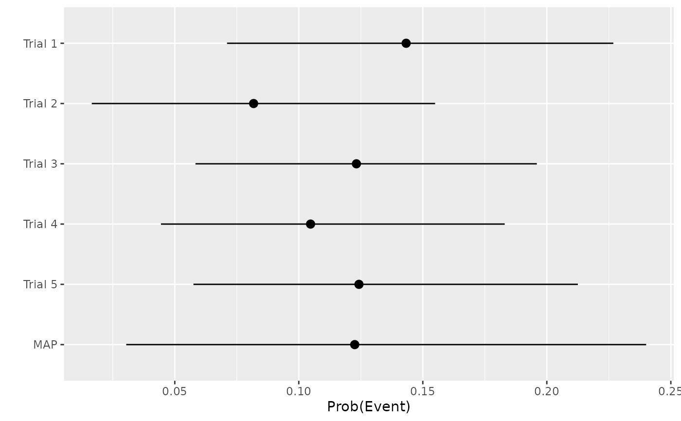
Create a forest-plot of MAP analysis.

Usage

forest_plot(x, alpha = 0.05, ...)

Arguments

x

Object of type bssd_binary_map.

alpha

0.05 to use 95% CIs, etc.

...

ignored.

Value

ggplot plot.

Examples

# Use a short MCMC run for this illustrative example.
check_iter <- 500
check_chains <- 1
set.seed(2021)
N <- 100
time <- 0.5 + cumsum(rexp(N, 100))
# Use constant hazard model:
hazard <- 0.15
prob <- 1 - exp(- hazard * time)
y <- rbinom(N, size = 1, prob = prob)
trial <- sample(1:5, size = N, replace = TRUE)
x <- stan_map_patient_data(y = y, trial = trial, time = time,
                           a_alpha = 1 / 3, a_beta = 1 / 3,
                           b_alpha = 5, b_beta = 5,
                           iter = check_iter, chains = check_chains,
                           refresh = 0)
#> Warning: Bulk Effective Samples Size (ESS) is too low, indicating posterior means and medians may be unreliable.
#> Running the chains for more iterations may help. See
#> https://mc-stan.org/misc/warnings.html#bulk-ess
#> Warning: Tail Effective Samples Size (ESS) is too low, indicating posterior variances and tail quantiles may be unreliable.
#> Running the chains for more iterations may help. See
#> https://mc-stan.org/misc/warnings.html#tail-ess
forest_plot(x)

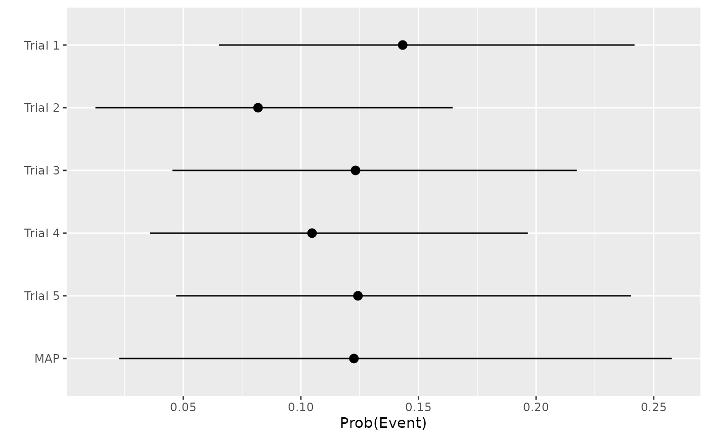forest_plot(x, alpha = 0.1)