Compare to publication
Compare_to_publication.RmdConsider the simulation scenarios from Table 3 of Zhao et al. (2024).
sim_scenario <- data.frame(Scenario = rep(1:12, each = 5),
                           Dose_level = paste0("Dose ", rep(1:5, 12)),
                           DLT = c(0.25, 0.41, 0.45, 0.49, 0.53,
                                   0.12, 0.25, 0.42, 0.49, 0.55,
                                   0.04, 0.12, 0.25, 0.43, 0.63,
                                   0.02, 0.06, 0.1,  0.25, 0.4,
                                   0.02, 0.05, 0.08, 0.11, 0.25,
                                   0.12, 0.25, 0.42, 0.49, 0.55,
                                   0.04, 0.12, 0.25, 0.43, 0.63,
                                   0.02, 0.06, 0.1,  0.25, 0.4,
                                   0.02, 0.05, 0.08, 0.11, 0.25,
                                   0.04, 0.12, 0.25, 0.43, 0.63,
                                   0.02, 0.06, 0.1,  0.25, 0.4,
                                   0.02, 0.05, 0.08, 0.11, 0.25),
                           Response = c(0.3,  0.4,  0.45, 0.5,  0.55,
                                        0.2,  0.3,  0.4,  0.5,  0.6,
                                        0.1,  0.2,  0.3,  0.45, 0.58,
                                        0.05, 0.1,  0.15, 0.3,  0.45,
                                        0.05, 0.1,  0.15, 0.2,  0.3,
                                        0.3,  0.35, 0.36, 0.36, 0.36,
                                        0.15, 0.3,  0.35, 0.36, 0.36,
                                        0.10, 0.2,  0.3,  0.35, 0.35,
                                        0.10, 0.15, 0.2,  0.3,  0.35,
                                        0.3,  0.32, 0.35, 0.36, 0.36,
                                        0.1,  0.3,  0.32, 0.35, 0.36,
                                        0.1,  0.15, 0.3,  0.32, 0.35))

tab_scenario <- sim_scenario |>
  tidyr::pivot_longer(cols = c("DLT", "Response"),
               names_to = "Rate",
               values_to = "value") |>
  tidyr::pivot_wider(names_from = Dose_level,
              values_from = "value")


knitr::kable(tab_scenario, row.names = NA)| Scenario | Rate | Dose 1 | Dose 2 | Dose 3 | Dose 4 | Dose 5 |
|---|---|---|---|---|---|---|
| 1 | DLT | 0.25 | 0.41 | 0.45 | 0.49 | 0.53 |
| 1 | Response | 0.30 | 0.40 | 0.45 | 0.50 | 0.55 |
| 2 | DLT | 0.12 | 0.25 | 0.42 | 0.49 | 0.55 |
| 2 | Response | 0.20 | 0.30 | 0.40 | 0.50 | 0.60 |
| 3 | DLT | 0.04 | 0.12 | 0.25 | 0.43 | 0.63 |
| 3 | Response | 0.10 | 0.20 | 0.30 | 0.45 | 0.58 |
| 4 | DLT | 0.02 | 0.06 | 0.10 | 0.25 | 0.40 |
| 4 | Response | 0.05 | 0.10 | 0.15 | 0.30 | 0.45 |
| 5 | DLT | 0.02 | 0.05 | 0.08 | 0.11 | 0.25 |
| 5 | Response | 0.05 | 0.10 | 0.15 | 0.20 | 0.30 |
| 6 | DLT | 0.12 | 0.25 | 0.42 | 0.49 | 0.55 |
| 6 | Response | 0.30 | 0.35 | 0.36 | 0.36 | 0.36 |
| 7 | DLT | 0.04 | 0.12 | 0.25 | 0.43 | 0.63 |
| 7 | Response | 0.15 | 0.30 | 0.35 | 0.36 | 0.36 |
| 8 | DLT | 0.02 | 0.06 | 0.10 | 0.25 | 0.40 |
| 8 | Response | 0.10 | 0.20 | 0.30 | 0.35 | 0.35 |
| 9 | DLT | 0.02 | 0.05 | 0.08 | 0.11 | 0.25 |
| 9 | Response | 0.10 | 0.15 | 0.20 | 0.30 | 0.35 |
| 10 | DLT | 0.04 | 0.12 | 0.25 | 0.43 | 0.63 |
| 10 | Response | 0.30 | 0.32 | 0.35 | 0.36 | 0.36 |
| 11 | DLT | 0.02 | 0.06 | 0.10 | 0.25 | 0.40 |
| 11 | Response | 0.10 | 0.30 | 0.32 | 0.35 | 0.36 |
| 12 | DLT | 0.02 | 0.05 | 0.08 | 0.11 | 0.25 |
| 12 | Response | 0.10 | 0.15 | 0.30 | 0.32 | 0.35 |
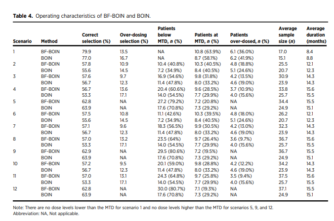
In the following chunk of code we use get.oc.bf to
calculate the operating characteristics of BF-BOIN under these
scenarios. In this vignette we only simulate 1000 trials per scenario,
and we only consider the first two scenarios.
generate_oc <- function(x, DLT_target = 0.25) {

  rate_dlt <- dplyr::filter(sim_scenario, Scenario == x)$DLT
  rate_response <- dplyr::filter(sim_scenario, Scenario == x)$Response

  temp <- get.oc.bf(ntrial = 1000,
                    seed = 1000,
                    target = DLT_target,
                    p.true = rate_dlt,
                    ncohort = 10,
                    cohortsize = 3,
                    n.earlystop = 9,
                    startdose = 1,
                    titration = FALSE,
                    p.saf = 0.6 * DLT_target,
                    p.tox = 1.4 * DLT_target,
                    cutoff.eli = 0.95,
                    extrasafe = FALSE,
                    offset = 0.05,
                    boundMTD=FALSE,
                    n.cap = 12,
                    end.backfill = TRUE,
                    n.per.month = 3,
                    dlt.window = 1,
                    p.response.true = rate_response,
                    three.plus.three = FALSE,
                    accrual = "uniform")


  out <- data.frame(Dose_level        = paste0("Dose ", 1:5),
                    Toxicity_rate     = rate_dlt,
                    Response_rate     = rate_response,
                    percent_selection = temp$selpercent,
                    n_patients        = temp$npatients,
                    percent_patients  = temp$percentpatients,
                    n_toxicity        = temp$ntox,
                    n_total           = temp$totaln,
                    percent_stop      = temp$percentstop,
                    duration          = temp$duration,
                    scenario          = x)

  return(out)
}

out_sim <- purrr::map_dfr(1:2, generate_oc)
head(out_sim)
#>       Dose_level Toxicity_rate Response_rate percent_selection n_patients
#> 1...1     Dose 1          0.25          0.30              79.7     11.251
#> 2...2     Dose 2          0.41          0.40              12.0      4.769
#> 3...3     Dose 3          0.45          0.45               0.6      0.707
#> 4...4     Dose 4          0.49          0.50               0.0      0.051
#> 5...5     Dose 5          0.53          0.55               0.1      0.012
#> 1...6     Dose 1          0.12          0.20              31.4     11.255
#>       percent_patients n_toxicity n_total percent_stop  duration scenario
#> 1...1      67.01012507      2.787  16.790          7.6  8.399349        1
#> 2...2      28.40381179      1.945  16.790          7.6  8.399349        1
#> 3...3       4.21083979      0.319  16.790          7.6  8.399349        1
#> 4...4       0.30375223      0.022  16.790          7.6  8.399349        1
#> 5...5       0.07147111      0.004  16.790          7.6  8.399349        1
#> 1...6      44.38441517      1.320  25.358          0.5 12.342858        2
Next we post-process this output to match the format of Table 4 of the paper.
out_OC <- out_sim |>
  dplyr::group_by(scenario, n_total, duration) |>
  dplyr::summarise(`Correct selection (%)`     = round(sum(percent_selection[Toxicity_rate == 0.25]), 1),
                   `Over-dosing selection (%)` = round(sum(percent_selection[Toxicity_rate > 0.25]), 1),
                   `Patients below MTD, n`     = sum(n_patients[Toxicity_rate < 0.25]),
                   `Patients below MTD, %`     = sum(percent_patients[Toxicity_rate < 0.25]),
                   `Patients at MTD, n`        = sum(n_patients[Toxicity_rate == 0.25]),
                   `Patients at MTD, %`        = sum(percent_patients[Toxicity_rate == 0.25]),
                   `Patients over-dosed, n`    = sum(n_patients[Toxicity_rate > 0.25]),
                   `Patients over-dosed, %`    = sum(percent_patients[Toxicity_rate > 0.25])) |>
  dplyr::mutate(`Patients below MTD, n (%)`    = paste0(round(`Patients below MTD, n`, 1),
                                                        " (", round(`Patients below MTD, %`, 1), ")"),
                `Patients at MTD, n (%)`       = paste0(round(`Patients at MTD, n`, 1),
                                                        " (", round(`Patients at MTD, %`, 1), ")"),
                `Patients over-dosed, n (%)`   = paste0(round(`Patients over-dosed, n`, 1),
                                                        " (", round(`Patients over-dosed, %`, 1), ")"),
                `Average sample size (n)`      = round(n_total, 1),
                `Average duration (months)`    = round(duration, 1)) |>
  dplyr::ungroup() |>
  dplyr::select(scenario, `Correct selection (%)`, `Over-dosing selection (%)`,
                `Patients below MTD, n (%)`, `Patients at MTD, n (%)`,
                `Patients over-dosed, n (%)`, `Average sample size (n)`,
                `Average duration (months)`)
#> `summarise()` has regrouped the output.
#> ℹ Summaries were computed grouped by scenario, n_total, and duration.
#> ℹ Output is grouped by scenario and n_total.
#> ℹ Use `summarise(.groups = "drop_last")` to silence this message.
#> ℹ Use `summarise(.by = c(scenario, n_total, duration))` for per-operation
#>   grouping (`?dplyr::dplyr_by`) instead.


knitr::kable(out_OC)| scenario | Correct selection (%) | Over-dosing selection (%) | Patients below MTD, n (%) | Patients at MTD, n (%) | Patients over-dosed, n (%) | Average sample size (n) | Average duration (months) |
|---|---|---|---|---|---|---|---|
| 1 | 79.7 | 12.7 | 0 (0) | 11.3 (67) | 5.5 (33) | 16.8 | 8.4 |
| 2 | 58.7 | 9.4 | 11.3 (44.4) | 10.3 (40.7) | 3.8 (15) | 25.4 | 12.3 |
And confirm that this matches (up to simulation error):