Calculate power for a multiple contrast test for a set of specified alternatives.
Usage
powMCT(
  contMat,
  alpha = 0.025,
  altModels,
  n,
  sigma,
  S,
  placAdj = FALSE,
  alternative = c("one.sided", "two.sided"),
  df,
  critV = TRUE,
  control = mvtnorm.control()
)
Arguments
- contMat
Contrast matrix to use. The individual contrasts should be saved in the columns of the matrix
- alpha
Significance level to use
- altModels
An object of class Mods, defining the mean vectors under which the power should be calculated
- n, sigma, S
Either a vector n and sigma or S need to be specified. When n and sigma are specified it is assumed computations are made for a normal homoscedastic ANOVA model with group sample sizes given by n and residual standard deviation sigma, i.e. the covariance matrix used for the estimates is thus
sigma^2*diag(1/n)and the degrees of freedom are calculated assum(n)-nrow(contMat). When a single number is specified for n it is assumed this is the sample size per group and balanced allocations are used.When S is specified this will be used as covariance matrix for the estimates.
- placAdj
Logical, if true, it is assumed that the standard deviation or variance matrix of the placebo-adjusted estimates are specified in sigma or S, respectively. The contrast matrix has to be produced on placebo-adjusted scale, see
optContr(), so that the coefficients are no longer contrasts (i.e. do not sum to 0).- alternative
Character determining the alternative for the multiple contrast trend test.
- df
Degrees of freedom to assume in case S (a general covariance matrix) is specified. When n and sigma are specified the ones from the corresponding ANOVA model are calculated.
- critV
Critical value, if equal to TRUE the critical value will be calculated. Otherwise one can directly specify the critical value here.
- control
A list specifying additional control parameters for the qmvt and pmvt calls in the code, see also mvtnorm.control for details.
References
Pinheiro J, Bornkamp B, Bretz F (2006). “Design and Analysis of Dose Finding Studies Combining Multiple Comparisons and Modeling Procedures.” Journal of Biopharmaceutical Statistics, 16, 639-656. doi:10.1080/10543400600860428 .
Examples
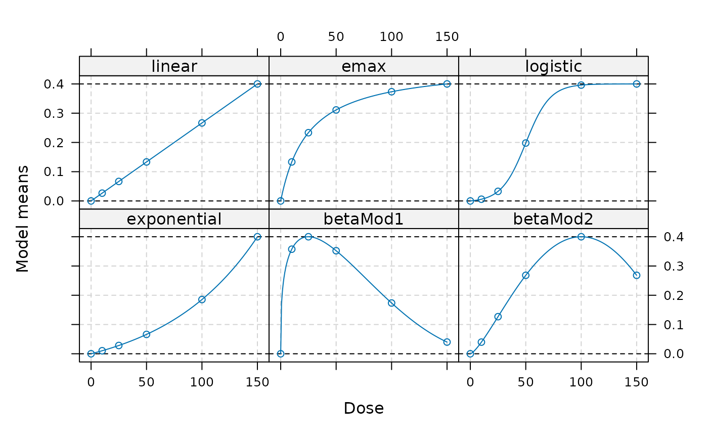
## look at power under some dose-response alternatives
## first the candidate models used for the contrasts
doses <- c(0,10,25,50,100,150)
## define models to use as alternative
fmodels <- Mods(linear = NULL, emax = 25,
                logistic = c(50, 10.88111), exponential= 85,
                betaMod=rbind(c(0.33,2.31),c(1.39,1.39)),
                doses = doses, addArgs=list(scal = 200),
                placEff = 0, maxEff = 0.4)
## plot alternatives
plot(fmodels)

## power for to detect a trend
contMat <- optContr(fmodels, w = 1)
powMCT(contMat, altModels = fmodels, n = 50, alpha = 0.05, sigma = 1)
#>      linear        emax    logistic exponential    betaMod1    betaMod2
#>   0.7015660   0.6849209   0.8519343   0.6711498   0.7338515   0.6775027

if (FALSE) { # \dontrun{
## power under the Dunnett test
## contrast matrix for Dunnett test with informative names
contMatD <- rbind(-1, diag(5))
rownames(contMatD) <- doses
colnames(contMatD) <- paste("D", doses[-1], sep="")
powMCT(contMatD, altModels = fmodels, n = 50, alpha = 0.05, sigma = 1)

## now investigate power of the contrasts in contMat under "general" alternatives
altFmods <- Mods(linInt = rbind(c(0, 1, 1, 1, 1),
                                  c(0.5, 1, 1, 1, 0.5)),
                 doses=doses, placEff=0, maxEff=0.5)
plot(altFmods)
powMCT(contMat, altModels = altFmods, n = 50, alpha = 0.05, sigma = 1)

## now the first example but assume information only on the
## placebo-adjusted scale
## for balanced allocations and 50 patients with sigma = 1 one obtains
## the following covariance matrix
S <- 1^2/50*diag(6)
## now calculate variance of placebo adjusted estimates
CC <- cbind(-1,diag(5))
V <- (CC)%*%S%*%t(CC)
linMat <- optContr(fmodels, doses = c(10,25,50,100,150),
                   S = V, placAdj = TRUE)
powMCT(linMat, altModels = fmodels, placAdj=TRUE,
       alpha = 0.05, S = V, df=6*50-6) # match df with the df above
} # }
## power for to detect a trend
contMat <- optContr(fmodels, w = 1)
powMCT(contMat, altModels = fmodels, n = 50, alpha = 0.05, sigma = 1)
#> linear emax logistic exponential betaMod1 betaMod2
#> 0.7015660 0.6849209 0.8519343 0.6711498 0.7338515 0.6775027
if (FALSE) { # \dontrun{
## power under the Dunnett test
## contrast matrix for Dunnett test with informative names
contMatD <- rbind(-1, diag(5))
rownames(contMatD) <- doses
colnames(contMatD) <- paste("D", doses[-1], sep="")
powMCT(contMatD, altModels = fmodels, n = 50, alpha = 0.05, sigma = 1)
## now investigate power of the contrasts in contMat under "general" alternatives
altFmods <- Mods(linInt = rbind(c(0, 1, 1, 1, 1),
c(0.5, 1, 1, 1, 0.5)),
doses=doses, placEff=0, maxEff=0.5)
plot(altFmods)
powMCT(contMat, altModels = altFmods, n = 50, alpha = 0.05, sigma = 1)
## now the first example but assume information only on the
## placebo-adjusted scale
## for balanced allocations and 50 patients with sigma = 1 one obtains
## the following covariance matrix
S <- 1^2/50*diag(6)
## now calculate variance of placebo adjusted estimates
CC <- cbind(-1,diag(5))
V <- (CC)%*%S%*%t(CC)
linMat <- optContr(fmodels, doses = c(10,25,50,100,150),
S = V, placAdj = TRUE)
powMCT(linMat, altModels = fmodels, placAdj=TRUE,
alpha = 0.05, S = V, df=6*50-6) # match df with the df above
} # }