Common multiple comparison procedures illustrated using graphicalMCP

library(graphicalMCP)

Introduction

In confirmatory clinical trials, regulatory guidelines mandate the strong control of the family-wise error rate at a prespecified level $\alpha$. Many multiple comparison procedures (MCPs) have been proposed for this purpose. The graphical approaches are a general framework that include many common MCPs as special cases. In this vignette, we illustrate how to use graphicalMCP to perform some common MCPs.

To test $m$ hypotheses using a graphical MCP, each hypothesis $H_i$ receives a weight $0\leq w_i\leq 1$ (called hypothesis weight), where $\sum_{i=1}^{m}w_i\leq 1$. From $H_i$ to $H_j$, there could be a directed and weighted edge $0\leq g_{ij}\leq 1$, which means that when $H_i$ is rejected, its hypothesis weight will be propagated (or transferred) to $H_j$ and $g_{ij}$ determines how much of the propagation. We also require $\sum_{j=1}^{m}g_{ij}\leq 1$ and $g_{ii}=0$.

Bonferroni-based procedures

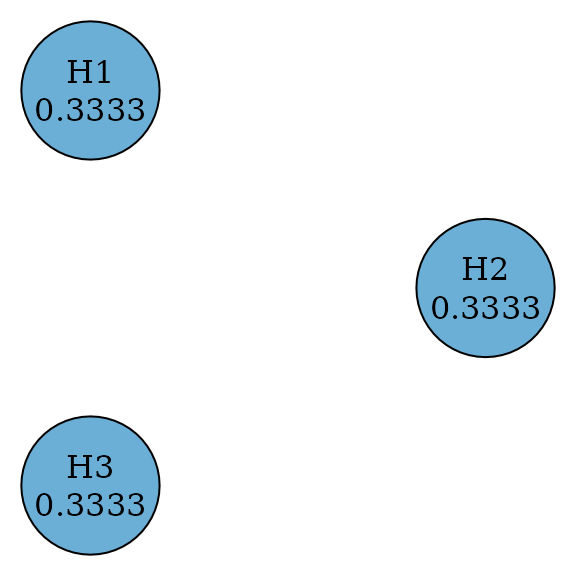
Bonferroni test

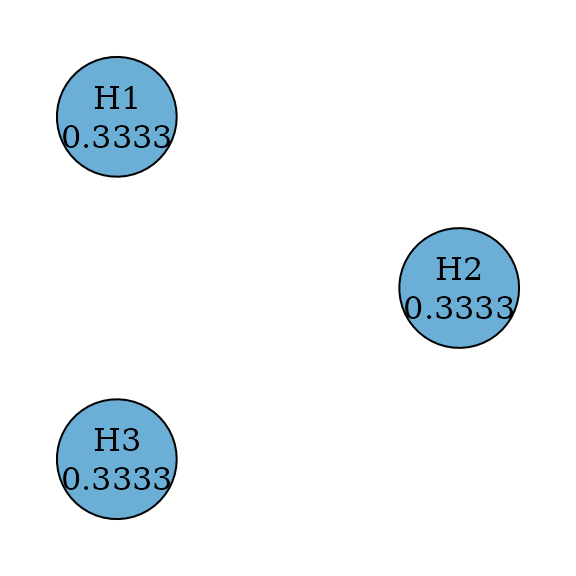
A Bonferroni test splits $\alpha$ equally among hypotheses by testing every hypothesis at a significance level of $\alpha$ divided by the number of hypotheses. Thus it rejects a hypothesis if its p-value is less than or equal to its significance level. There is no propagation between any pair of hypothesis.

set.seed(1234)
alpha <- 0.025
m <- 3
bonferroni_graph <- bonferroni(m)
# transitions <- matrix(0, m, m)
# bonferroni_graph <- graph_create(rep(1 / m, m), transitions)

plot(
  bonferroni_graph,
  layout = igraph::layout_in_circle(
    as_igraph(bonferroni_graph),
    order = c(2, 1, 3)
  ),
  vertex.size = 70
)

p_values <- runif(m, 0, alpha)

test_results <-
  graph_test_shortcut(
    bonferroni_graph,
    p = p_values,
    alpha = alpha
  )

test_results$outputs$rejected
#>    H1    H2    H3 
#>  TRUE FALSE FALSE

Weighted Bonferroni test

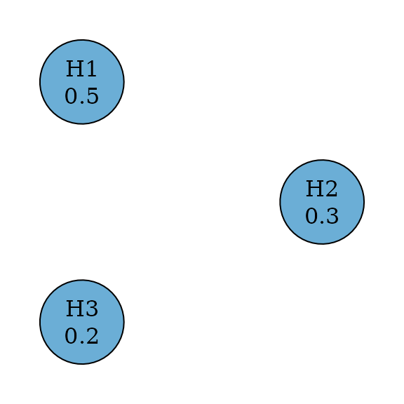
A weighted Bonferroni test splits $\alpha$ among hypotheses by testing every hypothesis at a significance level of $w_i\alpha$. Thus it rejects a hypothesis if its p-value is less than or equal to its significance level. When $w_i=w_j$ for all $i,j$, this means an equal split and the test is the Bonferroni test. There is no propagation between any pair of hypothesis.

set.seed(1234)
alpha <- 0.025
hypotheses <- c(0.5, 0.3, 0.2)
weighted_bonferroni_graph <- bonferroni_weighted(hypotheses)
# m <- length(hypotheses)
# transitions <- matrix(0, m, m)
# weighted_bonferroni_graph <- graph_create(hypotheses, transitions)

plot(
  weighted_bonferroni_graph,
  layout = igraph::layout_in_circle(
    as_igraph(bonferroni_graph),
    order = c(2, 1, 3)
  ),
  vertex.size = 70
)

p_values <- runif(m, 0, alpha)

test_results <-
  graph_test_shortcut(
    weighted_bonferroni_graph,
    p = p_values,
    alpha = alpha
  )

test_results$outputs$rejected
#>    H1    H2    H3 
#>  TRUE FALSE FALSE

Holm Procedure

Holm (or Bonferroni-Holm) procedures improve over Bonferroni tests by allowing propagation (Holm 1979). In other words, transition weights between hypotheses may not be zero. So it is uniformly more powerful than Bonferroni tests.

set.seed(1234)
alpha <- 0.025
m <- 3
holm_graph <- bonferroni_holm(m)
# transitions <- matrix(1 / (m - 1), m, m)
# diag(transitions) <- 0
# holm_graph <- graph_create(rep(1 / m, m), transitions)

plot(holm_graph,
  layout = igraph::layout_in_circle(
    as_igraph(holm_graph),
    order = c(2, 1, 3)
  ),
  vertex.size = 70
)

p_values <- runif(m, 0, alpha)

test_results <- graph_test_shortcut(holm_graph, p = p_values, alpha = alpha)

test_results$outputs$rejected
#>    H1    H2    H3 
#>  TRUE FALSE FALSE

Weighted Holm Procedure

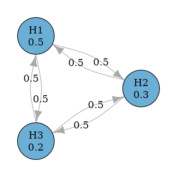
Weighted Holm (or weighted Bonferroni-Holm) procedures improve over weighted Bonferroni tests by allowing propagation (Holm 1979). In other words, transition weights between hypotheses may not be zero. So it is uniformly more powerful than weighted Bonferroni tests.

set.seed(1234)
alpha <- 0.025
hypotheses <- c(0.5, 0.3, 0.2)
weighted_holm_graph <- bonferroni_holm_weighted(hypotheses)
# m <- length(hypotheses)
# transitions <- matrix(1 / (m - 1), m, m)
# diag(transitions) <- 0
# weighted_holm_graph <- graph_create(hypotheses, transitions)

plot(weighted_holm_graph,
  layout = igraph::layout_in_circle(
    as_igraph(holm_graph),
    order = c(2, 1, 3)
  ),
  vertex.size = 70
)

p_values <- runif(m, 0, alpha)

test_results <- graph_test_shortcut(weighted_holm_graph, p = p_values, alpha = alpha)

test_results$outputs$rejected
#>    H1    H2    H3 
#>  TRUE FALSE FALSE

Fixed sequence procedure

Fixed sequence (or hierarchical) procedures pre-specify an order of testing Westfall and Krishen (2001). For example, the procedure will test $H_1$ first. If it is rejected, it will test $H_2$; otherwise the testing stops. If $H_2$ is rejected, it will test $H_3$; otherwise the testing stops. For each hypothesis, it will be tested at the full $\alpha$ level, when it can be tested.

set.seed(1234)
alpha <- 0.025
m <- 3
fixed_sequence_graph <- fixed_sequence(m)
# transitions <- rbind(
#   c(0, 1, 0),
#   c(0, 0, 1),
#   c(0, 0, 0)
# )
# fixed_sequence_graph <- graph_create(c(1, 0, 0), transitions)

plot(fixed_sequence_graph, nrow = 1, asp = 0.5, vertex.size = 50)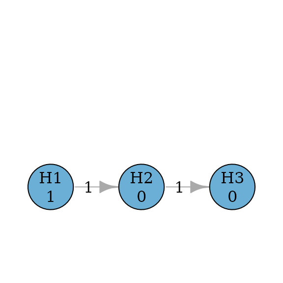

p_values <- runif(m, 0, alpha)

test_results <-
  graph_test_shortcut(
    fixed_sequence_graph,
    p = p_values,
    alpha = alpha
  )

test_results$outputs$rejected
#>   H1   H2   H3 
#> TRUE TRUE TRUE

Fallback procedure

Fallback procedures have one-way propagation (like fixed sequence procedures) but allow hypotheses to be tested at different significance levels (Wiens 2003).

set.seed(1234)
alpha <- 0.025
hypotheses <- c(0.5, 0.3, 0.2)
m <- length(hypotheses)
fallback_graph <- fallback(hypotheses)
# transitions <- rbind(
#   c(0, 1, 0),
#   c(0, 0, 1),
#   c(0, 0, 0)
# )
# fallback_graph <- graph_create(hypotheses, transitions)

plot(fallback_graph, nrow = 1, asp = 0.5, vertex.size = 50)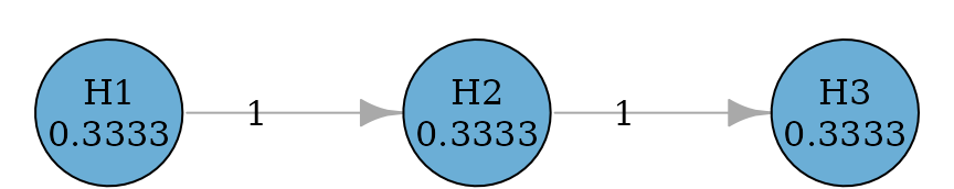

p_values <- runif(m, 0, alpha)

test_results <-
  graph_test_shortcut(
    fallback_graph,
    p = p_values,
    alpha = alpha
  )

test_results$outputs$rejected
#>   H1   H2   H3 
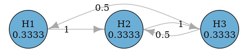
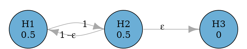
#> TRUE TRUE TRUE

Further they can be improved to allow propagation from later hypotheses to earlier hypotheses, because it is possible that a later hypothesis is rejected before an earlier hypothesis can be rejected. There are two versions of improvement: fallback_improved_1 due to Wiens and Dmitrienko (2005) and fallback_improved_2 due to Bretz et al. (2009) respectively.

set.seed(1234)
alpha <- 0.025
hypotheses <- c(0.5, 0.3, 0.2)
m <- length(hypotheses)
fallback_improved_1_graph <- fallback_improved_1(hypotheses)
# transitions <- rbind(
#   c(0, 1, 0),
#   c(0, 0, 1),
#   c(hypotheses[seq_len(m - 1)] / sum(hypotheses[seq_len(m - 1)]), 0)
# )
# fallback_improved_1_graph <- graph_create(hypotheses, transitions)
plot_layout <- rbind(
  c(0, 0.8),
  c(0.8, 0.8),
  c(0.4, 0)
)

plot(
  fallback_improved_1_graph,
  layout = plot_layout,
  asp = 0.5,
  edge_curves = c(pairs = 0.5),
  vertex.size = 70
)

epsilon <- 0.0001
fallback_improved_2_graph <- fallback_improved_2(hypotheses, epsilon)
# transitions <- rbind(
#   c(0, 1, 0),
#   c(1 - epsilon, 0, epsilon),
#   c(1, 0, 0)
# )
# fallback_improved_2_graph <- graph_create(hypotheses, transitions)
plot_layout <- rbind(
  c(0, 0.8),
  c(0.8, 0.8),
  c(0.4, 0)
)

plot(
  fallback_improved_2_graph,
  layout = plot_layout,
  eps = 0.0001,
  asp = 0.5,
  edge_curves = c(pairs = 0.5),
  vertex.size = 70
)

p_values <- runif(m, 0, alpha)

test_results <-
  graph_test_shortcut(
    fallback_improved_2_graph,
    p = p_values,
    alpha = alpha
  )

test_results$outputs$rejected
#>   H1   H2   H3 
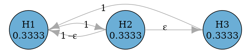
#> TRUE TRUE TRUE

Serial gatekeeping procedure

Serial gatekeeping procedures involve ordered multiple families of hypotheses, where all hypotheses of a family of hypotheses must be rejected before proceeding in the test sequence. The example below considers a primary family consisting of two hypotheses $H_1$ and $H_2$ and a secondary family consisting of a single hypothesis $H_3$. In the primary family, the Holm procedure is applied. If both $H_1$ and $H_2$ are rejected, $H_3$ can be tested at level $\alpha$; otherwise $H_3$ cannot be rejected. To allow the conditional propagation to $H_3$, an $\varepsilon$ edge is used from $H_2$ to $H_3$. It has a very small transition weight so that $H_2$ propagates most of its hypothesis weight to $H_1$ (if not already rejected) and retains a small (non-zero) weight for $H_3$ so that if $H_1$ has been rejected, all hypothesis weight of $H_2$ will be propagated to $H_3$. Here $\varepsilon$ is assigned to be 0.0001 and in practice, the value could be adjusted but it should be much smaller than the smallest p-value observed.

set.seed(1234)
alpha <- 0.025
m <- 3
epsilon <- 0.0001

transitions <- rbind(
  c(0, 1, 0),
  c(1 - epsilon, 0, epsilon),
  c(0, 0, 0)
)

serial_gatekeeping_graph <- graph_create(c(0.5, 0.5, 0), transitions)

plot_layout <- rbind(
  c(0, 0.8),
  c(0.8, 0.8),
  c(0.4, 0)
)

plot(
  serial_gatekeeping_graph,
  layout = plot_layout,
  eps = 0.0001,
  asp = 0.5,
  edge_curves = c(pairs = 0.5),
  vertex.size = 70
)

p_values <- runif(m, 0, alpha)

test_results <-
  graph_test_shortcut(
    serial_gatekeeping_graph,
    p = p_values,
    alpha = alpha
  )

test_results$outputs$rejected
#>   H1   H2   H3 
#> TRUE TRUE TRUE

Parallel gatekeeping procedure

Parallel gatekeeping procedures also involve multiple ordered families of hypotheses, where any null hypotheses of a family of hypotheses must be rejected before proceeding in the test sequence (Dmitrienko, Offen, and Westfall 2003). The example below considers a primary family consisting of two hypotheses $H_1$ and $H_2$ and a secondary family consisting of two hypotheses $H_3$ and $H_4$. In the primary family, the Bonferroni test is applied. If any of $H_1$ and $H_2$ is rejected, $H_3$ and $H_4$ can be tested at level $\alpha/2$ using the Holm procedure; if both $H_1$ and $H_2$ are rejected, $H_3$ and $H_4$ can be tested at level $\alpha$ using the Holm procedure; otherwise $H_3$ and $H_4$ cannot be rejected.

set.seed(1234)
alpha <- 0.025
m <- 4

transitions <- rbind(
  c(0, 0, 0.5, 0.5),
  c(0, 0, 0.5, 0.5),
  c(0, 0, 0, 1),
  c(0, 0, 1, 0)
)

parallel_gatekeeping_graph <- graph_create(c(0.5, 0.5, 0, 0), transitions)

plot(parallel_gatekeeping_graph, vertex.size = 70)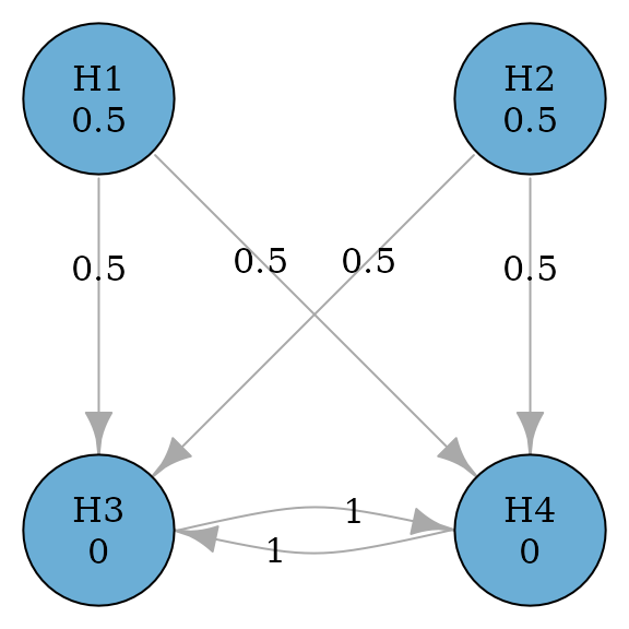

p_values <- runif(m, 0, alpha)

test_results <-
  graph_test_shortcut(
    parallel_gatekeeping_graph,
    p = p_values,
    alpha = alpha
  )

test_results$outputs$rejected
#>    H1    H2    H3    H4 
#>  TRUE FALSE FALSE FALSE

The above parallel gatekeeping procedure can be improved by adding $\varepsilon$ edges from secondary hypotheses to primary hypotheses, because it is possible that both secondary hypotheses are rejected but there is still a remaining primary hypothesis not rejected (Bretz et al. 2009).

set.seed(1234)
alpha <- 0.025
m <- 4
epsilon <- 0.0001

transitions <- rbind(
  c(0, 0, 0.5, 0.5),
  c(0, 0, 0.5, 0.5),
  c(epsilon, 0, 0, 1 - epsilon),
  c(0, epsilon, 1 - epsilon, 0)
)

parallel_gatekeeping_improved_graph <-
  graph_create(c(0.5, 0.5, 0, 0), transitions)

plot(parallel_gatekeeping_improved_graph, eps = 0.0001, vertex.size = 70)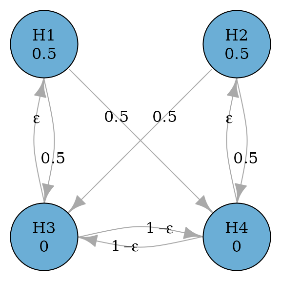

p_values <- runif(m, 0, alpha)

test_results <-
  graph_test_shortcut(
    parallel_gatekeeping_improved_graph,
    p = p_values,
    alpha = alpha
  )

test_results$outputs$rejected
#>    H1    H2    H3    H4 
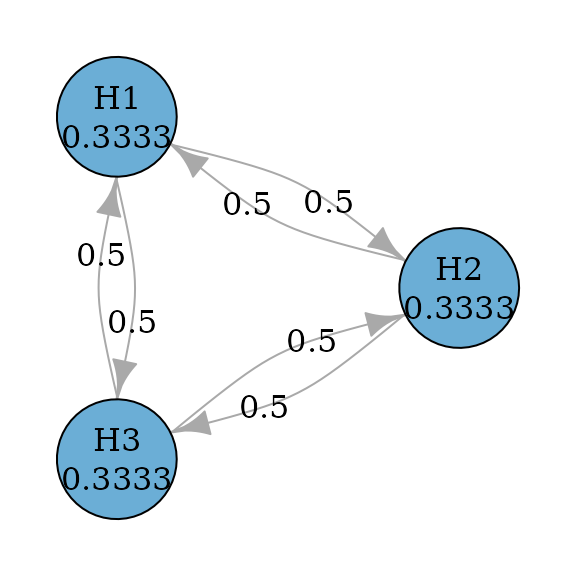
#>  TRUE FALSE FALSE FALSE

Successive procedure

Successive procedures incorporate successive relationships between hypotheses. For example, the secondary hypothesis is not tested until the primary hypothesis has been rejected. This is similar to using the fixed sequence procedure as a component of a graph. The example below considers two primary hypotheses $H_1$ and $H_2$ and two secondary hypotheses $H_3$ and $H_4$. Primary hypotheses $H_1$ and $H_2$ receive the equal hypothesis weight of 0.5; secondary hypotheses $H_3$ and $H_4$ receive the hypothesis weight of 0. A secondary hypothesis $H_3 (H_4)$ can be tested only if the corresponding primary hypothesis $H_1 (H_2)$ has been rejected. This represents the successive relationships between $H_1$ and $H_3$, and $H_2$ and $H_4$, respectively (Maurer, Glimm, and Bretz 2011). If both $H_1$ and $H_3$ are rejected, their hypothesis weights are propagated to $H_2$ and $H_4$, and vice versa.

set.seed(1234)
alpha <- 0.025
m <- 4
simple_successive_graph <- simple_successive_1()
# transitions <- rbind(
#   c(0, 0, 1, 0),
#   c(0, 0, 0, 1),
#   c(0, 1, 0, 0),
#   c(1, 0, 0, 0)
# )
# simple_successive_graph <- graph_create(c(0.5, 0.5, 0, 0), transitions)

plot(simple_successive_graph, layout = "grid", nrow = 2, vertex.size = 70)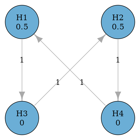

p_values <- runif(m, 0, alpha)

test_results <-
  graph_test_shortcut(
    simple_successive_graph,
    p = p_values,
    alpha = alpha
  )

test_results$outputs$rejected
#>    H1    H2    H3    H4 
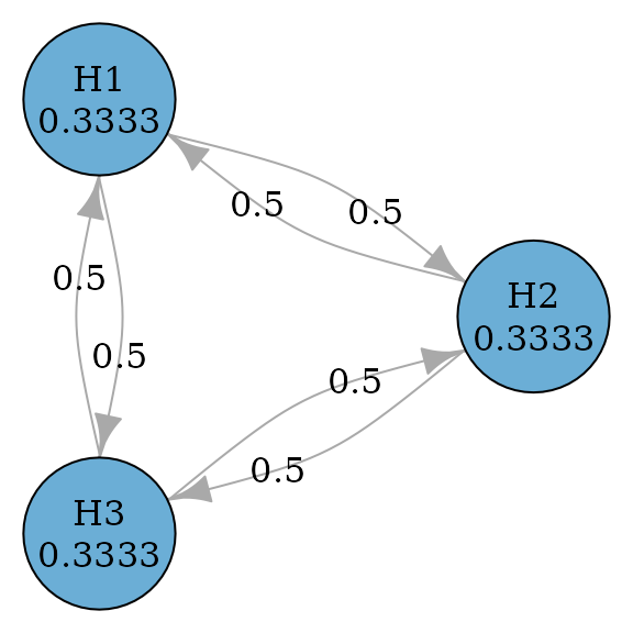
#>  TRUE FALSE FALSE FALSE

The above graph could be generalized to allow propagation between primary hypotheses (Maurer, Glimm, and Bretz 2011). A general successive graph is illustrate below with a variable to determine the propagation between $H_1$ and $H_2$.

set.seed(1234)
alpha <- 0.025
m <- 4

successive_var <- simple_successive_var <- function(gamma) {
  graph_create(
    c(0.5, 0.5, 0, 0),
    rbind(
      c(0, gamma, 1 - gamma, 0),
      c(gamma, 0, 0, 1 - gamma),
      c(0, 1, 0, 0),
      c(1, 0, 0, 0)
    )
  )
}

successive_var_graph <- successive_var(0.5)
plot(successive_var_graph, layout = "grid", nrow = 2, vertex.size = 70)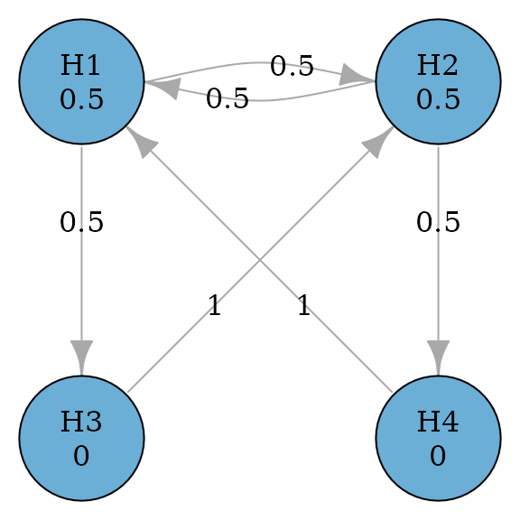

p_values <- runif(m, 0, alpha)

test_results <-
  graph_test_shortcut(
    successive_var_graph,
    p = p_values,
    alpha = alpha
  )

test_results$outputs$rejected
#>    H1    H2    H3    H4 
#>  TRUE  TRUE FALSE FALSE

Hochberg-based procedures

Hochberg procedure

Hochberg procedure (Hochberg 1988) is a closed test procedure which uses Hochberg tests for every intersection hypothesis. According to Xi and Bretz (2019), the graph for Hochberg procedures is the same as the graph for Holm procedures. Thus to perform Hochberg procedure, we just need to specify test_type to be hochberg.

set.seed(1234)
alpha <- 0.025
m <- 3
hochberg_graph <- hochberg(m)

plot(
  hochberg_graph,
  layout = igraph::layout_in_circle(
    as_igraph(hochberg_graph),
    order = c(2, 1, 3)
  ),
  vertex.size = 70
)

p_values <- runif(m, 0, alpha)

test_results <- graph_test_closure(
  hochberg_graph,
  p = p_values,
  alpha = alpha,
  test_types = "hochberg"
)

test_results$outputs$rejected
#>   H1   H2   H3 
#> TRUE TRUE TRUE

Simes-based procedures

Hommel procedure

Hommel procedure (Hommel 1988) is a closed test procedure which uses Simes tests for every intersection hypothesis. According to Xi and Bretz (2019), the graph for Hommel procedures is the same as the graph for Holm procedures. Thus to perform Hommel procedure, we just need to specify test_type to be simes.

set.seed(1234)
alpha <- 0.025
m <- 3
hommel_graph <- hommel(m)

plot(
  hommel_graph,
  layout = igraph::layout_in_circle(
    as_igraph(hommel_graph),
    order = c(2, 1, 3)
  ),
  vertex.size = 70
)

p_values <- runif(m, 0, alpha)

test_results <- graph_test_closure(
  hommel_graph,
  p = p_values,
  alpha = alpha,
  test_types = "simes"
)

test_results$outputs$rejected
#>   H1   H2   H3 
#> TRUE TRUE TRUE

Parametric procedures

Šidák test

The Šidák test is similar to the equally weighted Bonferroni test but it assumes test statistics are independent of each other (Šidák 1967). Thus it can be performed as a parametric procedure with the identity correlation matrix. Its graph is the same as the graph for the equally weighted Bonferroni test.

set.seed(1234)
alpha <- 0.025
m <- 3
sidak_graph <- sidak(m)

plot(
  sidak_graph,
  layout = igraph::layout_in_circle(
    as_igraph(bonferroni_graph),
    order = c(2, 1, 3)
  ),
  vertex.size = 70
)

p_values <- runif(m, 0, alpha)
corr <- diag(m)

test_results <- graph_test_closure(
  sidak_graph,
  p = p_values, alpha = alpha,
  test_types = "parametric",
  test_corr = list(corr)
)

test_results$outputs$rejected
#>    H1    H2    H3 
#>  TRUE FALSE FALSE

Dunnett test

Single-step Dunnett tests are an improvement from Bonferroni tests by incorporating the correlation structure between test statistics (Dunnett 1955). Thus their graphs are the same as Bonferroni tests. Assume an equi-correlated case, where the correlation between any pair of test statistics is the same, e.g., 0.5. Then we can perform the single-step Dunnett test by specifying test_type to be parametric and providing the correlation matrix.

set.seed(1234)
alpha <- 0.025
m <- 3
dunnett_graph <- dunnett_single_step(m)

plot(
  dunnett_graph,
  layout = igraph::layout_in_circle(
    as_igraph(dunnett_graph),
    order = c(2, 1, 3)
  ),
  vertex.size = 70
)

p_values <- runif(m, 0, alpha)
corr <- matrix(0.5, m, m)
diag(corr) <- 1

test_results <- graph_test_closure(
  dunnett_graph,
  p = p_values, alpha = alpha,
  test_types = "parametric",
  test_corr = list(corr)
)

test_results$outputs$rejected
#>    H1    H2    H3 
#>  TRUE FALSE FALSE

Weighted Dunnett test

Weighted single-step Dunnett tests are an improvement from weighted Bonferroni tests by incorporating the correlation structure between test statistics (Xi et al. 2017). Thus their graphs are the same as weighted Bonferroni tests. Assume an equi-correlated case, where the correlation between any pair of test statistics is the same, e.g., 0.5. Then we can perform the weighted single-step Dunnett test by specifying test_type to be parametric and providing the correlation matrix.

set.seed(1234)
alpha <- 0.025
hypotheses <- c(0.5, 0.3, 0.2)
dunnett_graph <- dunnett_single_step_weighted(hypotheses)

plot(
  dunnett_graph,
  layout = igraph::layout_in_circle(
    as_igraph(dunnett_graph),
    order = c(2, 1, 3)
  ),
  vertex.size = 70
)

p_values <- runif(m, 0, alpha)
corr <- matrix(0.5, m, m)
diag(corr) <- 1

test_results <- graph_test_closure(
  dunnett_graph,
  p = p_values, alpha = alpha,
  test_types = "parametric",
  test_corr = list(corr)
)

test_results$outputs$rejected
#>    H1    H2    H3 
#>  TRUE FALSE FALSE

Dunnett procedure

Dunnett procedures are a closed test procedure and an improvement from Holm procedures by incorporating the correlation structure between test statistics (Xi et al. 2017). Thus their graphs are the same as Holm procedures. Assume an equi-correlated case, where the correlation between any pair of test statistics is the same, e.g., 0.5. Then we can perform the step-down Dunnett procedure by specifying test_type to be parametric and providing the correlation matrix.

set.seed(1234)
alpha <- 0.025
hypotheses <- c(0.5, 0.3, 0.2)
dunnett_graph <- dunnett_closure_weighted(hypotheses)

plot(
  dunnett_graph,
  layout = igraph::layout_in_circle(
    as_igraph(dunnett_graph),
    order = c(2, 1, 3)
  ),
  vertex.size = 70
)

p_values <- runif(m, 0, alpha)
corr <- matrix(0.5, m, m)
diag(corr) <- 1

test_results <- graph_test_closure(
  dunnett_graph,
  p = p_values, alpha = alpha,
  test_types = "parametric",
  test_corr = list(corr)
)

test_results$outputs$rejected
#>    H1    H2    H3 
#>  TRUE FALSE FALSE

Reference

Bretz, Frank, Willi Maurer, Werner Branath, and Martin Posch. 2009. “A Graphical Approach to Sequentially Rejective Multiple Test Procedures.” Statistics in Medicine 53 (4): 586–604. https://doi.org/10.1002/sim.3495.

Dmitrienko, Alexei, Walter W. Offen, and Peter H. Westfall. 2003. “Gatekeeping Strategies for Clinical Trials That Do Not Require All Primary Effects to Be Significant.” Statistics in Medicine 22 (15): 2387–2400. https://doi.org/10.1002/sim.1526.

Dunnett, Charles W. 1955. “A Multiple Comparison Procedure for Comparing Several Treatments with a Control.” Journal of the American Statistical Association 50 (272): 1096–1121.

Hochberg, Yosef. 1988. “A Sharper Bonferroni Procedure for Multiple Tests of Significance.” Biometrika 75 (4): 800–802.

Holm, Sture. 1979. “A Simple Sequentially Rejective Multiple Test Procedure.” Scandinavian Journal of Statistics 75: 65–70.

Hommel, Gerhard. 1988. “A Stagewise Rejective Multiple Test Procedure Based on a Modified Bonferroni Test.” Biometrika 75 (2): 383–86. https://doi.org/10.1093/biomet/75.2.383.

Maurer, Willi, Ekkehard Glimm, and Frank Bretz. 2011. “Multiple and Repeated Testing of Primary, Coprimary, and Secondary Hypotheses.” Statistics in Biopharmaceutical Research 3 (2): 336–52. https://doi.org/10.1198/sbr.2010.10010.

Maurer, Willi, Ludwig Hothorn, and Walter Lehmacher. 1995. “Multiple Comparisons in Drug Clinical Trials and Preclinical Assays: A-Priori Ordered Hypotheses.” Biometrie in Der Chemisch-Pharmazeutischen Industrie 6: 3–18.

Šidák, Zbyněk. 1967. “Rectangular Confidence Regions for the Means of Multivariate Normal Distributions.” Journal of the American Statistical Association 62 (318): 626–33.

Westfall, Peter H., and Alok Krishen. 2001. “Optimally Weighted, Fixed Sequence and Gatekeeper Multiple Testing Procedures.” Journal of Statistical Planning and Inference 99 (1): 25–40. https://doi.org/10.1016/S0378-3758(01)00077-5.

Wiens, Brian L. 2003. “A Fixed Sequence Bonferroni Procedure for Testing Multiple Endpoints.” Pharmaceutical Statistics 2 (3): 211–15. https://doi.org/10.1002/pst.64.

Wiens, Brian L., and Alexei Dmitrienko. 2005. “The Fallback Procedure for Evaluating a Aingle Family of Hypotheses.” Journal of Biopharmaceutical Statistics 15 (6): 929–42. https://doi.org/10.1080/10543400500265660.

Xi, Dong, and Frank Bretz. 2019. “Symmetric Graphs for Equally Weighted Tests, with Application to the Hochberg Procedure.” Statistics in Medicine 38 (27): 5268–82. https://doi.org/10.1002/sim.8375.

Xi, Dong, Ekkehard Glimm, Willi Maurer, and Frank Bretz. 2017. “A Unified Framework for Weighted Parametric Multiple Test Procedures.” Biometrical Journal 59 (5): 918–31. https://doi.org/10.1002/bimj.201600233.