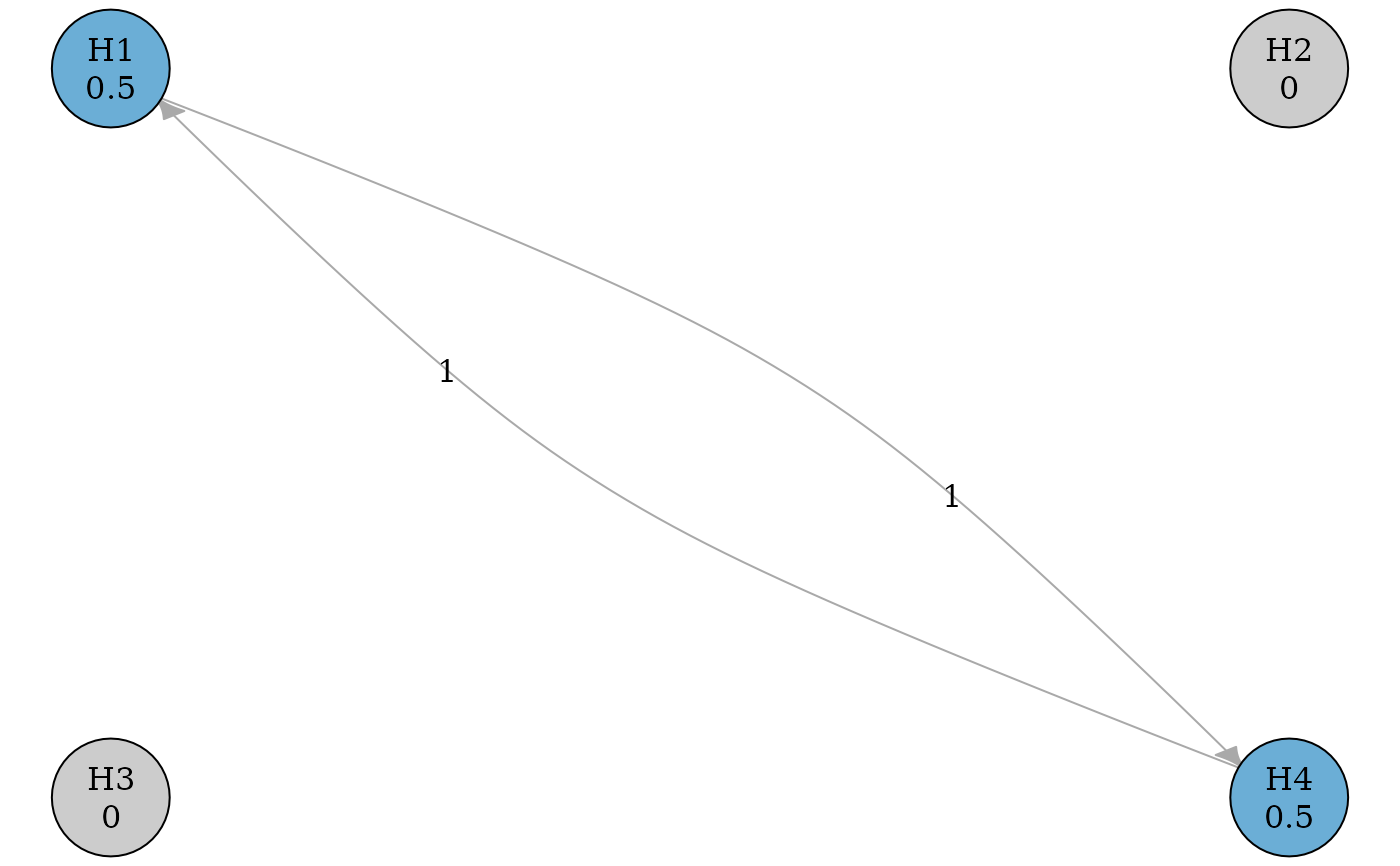
Plotting an updated graph is a very light wrapper around
plot.initial_graph(), only changing the default vertex color to use gray
for deleted hypotheses.
Usage
# S3 method for class 'updated_graph'
plot(x, ...)
Arguments
- x
An object of class
updated_graphto plot.- ...
Arguments passed on to
plot.initial_graphv_paletteA character vector of length two specifying the colors for retained and deleted hypotheses. More extensive color customization must be done with
vertex.color.layoutAn igraph layout specification (See
?igraph.plotting), or"grid", which lays out hypotheses left-to-right and top-to-bottom.nrowandncolcontrol the grid shape.nrowAn integer scalar specifying the number of rows in the vertex grid. If row and column counts are not specified, vertices will be laid out as close to a square as possible.
ncolAn integer scalar specifying the number of columns in the vertex grid. If row and column counts are not specified, vertices will be laid out as close to a square as possible.
edge_curvesA named numeric vector specifying the curvature of specific edges. Edge pairs (Where two vertices share an edge in each possible direction) are detected automatically and get 0.25 curvature. Adjust edges by adding an entry with name
"vertex1|vertex2, and adjust default edge pairs curvature by adding an entry with name"pairs"-edge_curves = c("pairs" = 0.5, "H1|H3" = 0.25, "H3|H4" = 0.75).precisionAn integer scalar indicating the number of decimal places to display.
epsA numeric scalar. The transition weight of
epswill be displayed as \(\epsilon\), which indicates edges with infinitesimally small weights. See Bretz et al. (2009) for more details.background_colorA character scalar specifying a background color for the whole plotting area. Passed directly to
graphics::par()(bg).marginsA length 4 numeric vector specifying the margins for the plot. Defaults to all 1, since igraph plots tend to have large margins. It is passed directly to
graphics::par()(mar).
References
Bretz, F., Posch, M., Glimm, E., Klinglmueller, F., Maurer, W., and Rohmeyer, K. (2011). Graphical approaches for multiple comparison procedures using weighted Bonferroni, Simes, or parametric tests. Biometrical Journal, 53(6), 894-913.
See also
plot.initial_graph() for the plot method for the initial graph.
Examples
# A graphical multiple comparison procedure with two primary hypotheses (H1
# and H2) and two secondary hypotheses (H3 and H4)
# See Figure 1 in Bretz et al. (2011).
hypotheses <- c(0.5, 0.5, 0, 0)
transitions <- rbind(
  c(0, 0, 1, 0),
  c(0, 0, 0, 1),
  c(0, 1, 0, 0),
  c(1, 0, 0, 0)
)
g <- graph_create(hypotheses, transitions)

# Delete the second and third hypotheses in the "unordered mode"
plot(
  graph_update(
    g,
    c(FALSE, TRUE, TRUE, FALSE)
  ),
  layout = "grid"
)

