Introduction
In this vignette we briefly compare the mmrm::mmrm,
SAS’s PROC GLIMMIX, nlme::gls,
lme4::lmer, and glmmTMB::glmmTMB functions for
fitting mixed models for repeated measures (MMRMs). A primary difference
in these implementations lies in the covariance structures that are
supported “out of the box”. In particular, PROC GLIMMIX and
mmrm are the only procedures which provide support for many
of the most common MMRM covariance structures. Most covariance
structures can be implemented in gls, though users are
required to define them manually. lmer and
glmmTMB are more limited. We find that mmmrm
converges more quickly than other R implementations while also producing
estimates that are virtually identical to
PROC GLIMMIX’s.
Datasets
Two datasets are used to illustrate model fitting with the
mmrm, lme4, nlme,
glmmTMB R packages as well as PROC GLIMMIX.
These data are also used to compare these implementations’ operating
characteristics.
FEV Data
The FEV dataset contains measurements of FEV1 (forced expired volume in one second), a measure of how quickly the lungs can be emptied. Low levels of FEV1 may indicate chronic obstructive pulmonary disease (COPD). It is summarized below.
                                      Stratified by ARMCD
                               Overall       PBO           TRT
  n                              800           420           380
  USUBJID (%)
     PT[1-200]                   200           105 (52.5)     95 (47.5)
  AVISIT
     VIS1                        200           105            95
     VIS2                        200           105            95
     VIS3                        200           105            95
     VIS4                        200           105            95
  RACE (%)
     Asian                       280 (35.0)    152 (36.2)    128 (33.7)
     Black or African American   300 (37.5)    184 (43.8)    116 (30.5)
     White                       220 (27.5)     84 (20.0)    136 (35.8)
  SEX = Female (%)               424 (53.0)    220 (52.4)    204 (53.7)
  FEV1_BL (mean (SD))          40.19 (9.12)  40.46 (8.84)  39.90 (9.42)
  FEV1 (mean (SD))             42.30 (9.32)  40.24 (8.67)  44.45 (9.51)
  WEIGHT (mean (SD))            0.52 (0.23)   0.52 (0.23)   0.51 (0.23)
  VISITN (mean (SD))            2.50 (1.12)   2.50 (1.12)   2.50 (1.12)
  VISITN2 (mean (SD))          -0.02 (1.03)   0.01 (1.07)  -0.04 (0.98)
BCVA Data
The BCVA dataset contains data from a randomized longitudinal ophthalmology trial evaluating the change in baseline corrected visual acuity (BCVA) over the course of 10 visits. BCVA corresponds to the number of letters read from a visual acuity chart. A summary of the data is given below:
                                      Stratified by ARMCD
                               Overall         CTL            TRT
  n                             8605          4123           4482
  USUBJID (%)
     PT[1-1000]                 1000           494 (49.4)     506 (50.6)
  AVISIT
     VIS1                        983           482            501
     VIS2                        980           481            499
     VIS3                        960           471            489
     VIS4                        946           458            488
     VIS5                        925           454            471
     VIS6                        868           410            458
     VIS7                        816           388            428
     VIS8                        791           371            420
     VIS9                        719           327            392
     VIS10                       617           281            336
  RACE (%)
     Asian                       297 (29.7)    151 (30.6)     146 (28.9)
     Black or African American   317 (31.7)    149 (30.1)     168 (33.2)
     White                       386 (38.6)    194 (39.3)     192 (37.9)
  BCVA_BL (mean (SD))          75.12 (9.93)  74.90 (9.76)   75.40 (10.1)
  BCVA_CHG (mean (SD))
     VIS1                       5.59 (1.31)   5.32 (1.23)    5.86 (1.33)
     VIS10                      9.18 (2.91)   7.49 (2.58)   10.60 (2.36)
Model Implementations
Listed below are some of the most commonly used covariance structures
used when fitting MMRMs. We indicate which matrices are available “out
of the box” for each implementation considered in this vignette. Note
that this table is not exhaustive; PROC GLIMMIX and
glmmTMB support additional spatial covariance
structures.
| Covariance structures | mmrm |
PROC GLIMMIX |
gls |
lmer |
glmmTMB |
|---|---|---|---|---|---|
| Ante-dependence (heterogeneous) | X | X | |||
| Ante-dependence (homogeneous) | X | ||||
| Auto-regressive (heterogeneous) | X | X | X | ||
| Auto-regressive (homogeneous) | X | X | X | X | |
| Compound symmetry (heterogeneous) | X | X | X | X | |
| Compound symmetry (homogeneous) | X | X | X | ||
| Spatial exponential | X | X | X | X | |
| Toeplitz (heterogeneous) | X | X | X | ||
| Toeplitz (homogeneous) | X | X | |||
| Unstructured | X | X | X | X | X |
Code for fitting MMRMs to the FEV data using each of the considered functions and covariance structures are provided below. Fixed effects for the visit number, treatment assignment and the interaction between the two are modeled.
Ante-dependence (heterogeneous)
PROC GLIMMIX
PROC GLIMMIX DATA = fev_data;
CLASS AVISIT(ref = 'VIS1') ARMCD(ref = 'PBO') USUBJID;
MODEL FEV1 = AVISIT|ARMCD / ddfm=satterthwaite solution chisq;
RANDOM AVISIT / subject=USUBJID type=ANTE(1);
mmrm
mmrm(
  formula = FEV1 ~ ARMCD * AVISIT + adh(VISITN | USUBJID),
  data = fev_data
)
Ante-dependence (homogeneous)
mmrm
mmrm(
  formula =FEV1 ~ ARMCD * AVISIT + ad(VISITN | USUBJID),
  data = fev_data
)
Auto-regressive (heterogeneous)
PROC GLIMMIX
PROC GLIMMIX DATA = fev_data;
CLASS AVISIT(ref = 'VIS1') ARMCD(ref = 'PBO') USUBJID;
MODEL FEV1 = AVISIT|ARMCD / ddfm=satterthwaite solution chisq;
RANDOM AVISIT / subject=USUBJID type=ARH(1);
mmrm
mmrm(
  formula = FEV1 ~ ARMCD * AVISIT + ar1h(VISITN | USUBJID),
  data = fev_data
)Auto-regressive (homogeneous)
PROC GLIMMIX
PROC GLIMMIX DATA = fev_data;
CLASS AVISIT(ref = 'VIS1') ARMCD(ref = 'PBO') USUBJID;
MODEL FEV1 =  ARMCD|AVISIT / ddfm=satterthwaite solution chisq;
RANDOM AVISIT / subject=USUBJID type=AR(1);
mmrm
mmrm(
  formula = FEV1 ~ ARMCD * AVISIT + ar1(VISITN | USUBJID),
  data = fev_data
)Compound symmetry (heterogeneous)
PROC GLIMMIX
PROC GLIMMIX DATA = fev_data;
CLASS AVISIT(ref = 'VIS1') ARMCD(ref = 'PBO') USUBJID;
MODEL FEV1 = AVISIT|ARMCD / ddfm=satterthwaite solution chisq;
RANDOM AVISIT / subject=USUBJID type=CSH;
mmrm
mmrm(
  formula = FEV1 ~ ARMCD * AVISIT + csh(VISITN | USUBJID),
  data = fev_data
)Compound symmetry (homogeneous)
PROC GLIMMIX
PROC GLIMMIX DATA = fev_data;
CLASS AVISIT(ref = 'VIS1') ARMCD(ref = 'PBO') USUBJID;
MODEL FEV1 = AVISIT|ARMCD / ddfm=satterthwaite solution chisq;
RANDOM AVISIT / subject=USUBJID type=CS;
mmrm
mmrm(
  formula = FEV1 ~ ARMCD * AVISIT + cs(VISITN | USUBJID),
  data = fev_data
)Spatial exponential
PROC GLIMMIX
PROC GLIMMIX DATA = fev_data;
CLASS AVISIT(ref = 'VIS1') ARMCD(ref = 'PBO') USUBJID;
MODEL FEV1 = AVISIT|ARMCD / ddfm=satterthwaite solution chisq;
RANDOM / subject=USUBJID type=sp(exp)(visitn) rcorr;
mmrm
mmrm(
  formula = FEV1 ~ ARMCD * AVISIT + sp_exp(VISITN | USUBJID),
  data = fev_data
)
gls
gls(
  FEV1 ~ ARMCD * AVISIT,
  data = fev_data,
  correlation = corExp(form = ~AVISIT | USUBJID),
  weights = varIdent(form = ~1|AVISIT),
  na.action = na.omit
)
glmmTMB
# NOTE: requires use of coordinates
glmmTMB(
  FEV1 ~ ARMCD * AVISIT + exp(0 + AVISIT | USUBJID),
  dispformula = ~ 0,
  data = fev_data
)
Toeplitz (heterogeneous)
PROC GLIMMIX
PROC GLIMMIX DATA = fev_data;
CLASS AVISIT(ref = 'VIS1') ARMCD(ref = 'PBO') USUBJID;
MODEL FEV1 = AVISIT|ARMCD / ddfm=satterthwaite solution chisq;
RANDOM AVISIT / subject=USUBJID type=TOEPH;
mmrm
mmrm(
  formula = FEV1 ~ ARMCD * AVISIT + toeph(AVISIT | USUBJID),
  data = fev_data
)Toeplitz (homogeneous)
PROC GLIMMIX
PROC GLIMMIX DATA = fev_data;
CLASS AVISIT(ref = 'VIS1') ARMCD(ref = 'PBO') USUBJID;
MODEL FEV1 = AVISIT|ARMCD / ddfm=satterthwaite solution chisq;
RANDOM AVISIT / subject=USUBJID type=TOEP;
mmrm
mmrm(
  formula = FEV1 ~ ARMCD * AVISIT + toep(AVISIT | USUBJID),
  data = fev_data
)
Unstructured
PROC GLIMMIX
PROC GLIMMIX DATA = fev_data;
CLASS AVISIT(ref = 'VIS1') ARMCD(ref = 'PBO') USUBJID;
MODEL FEV1 = ARMCD|AVISIT / ddfm=satterthwaite solution chisq;
RANDOM AVISIT / subject=USUBJID type=un;
mmrm
mmrm(
  formula = FEV1 ~ ARMCD * AVISIT + us(AVISIT | USUBJID),
  data = fev_data
)
gls
gls(
  FEV1 ~  ARMCD * AVISIT,
  data = fev_data,
  correlation = corSymm(form = ~AVISIT | USUBJID),
  weights = varIdent(form = ~1|AVISIT),
  na.action = na.omit
)Benchmarking
Next, the MMRM fitting procedures are compared using the FEV and BCVA datasets. FEV1 measurements are modeled as a function of race, treatment arm, visit number, and the interaction between the treatment arm and the visit number. Change in BCVA is assumed to be a function of race, baseline BCVA, treatment arm, visit number, and the treatment–visit interaction. In both datasets, repeated measures are modeled using an unstructured covariance matrix. The implementations’ convergence times are evaluated first, followed by a comparison of their estimates. Finally, we fit these procedures on simulated BCVA-like data to assess the impact of missingness on convergence rates.
Convergence Times
FEV Data
The mmrm, PROC GLIMMIX, gls,
lmer, and glmmTMB functions are applied to the
FEV dataset 10 times. The convergence times are recorded for each
replicate and are reported in the table below.
| Implementation | Median | First Quartile | Third Quartile |
|---|---|---|---|
| mmrm | 56.15 | 55.76 | 56.30 |
| PROC GLIMMIX | 100.00 | 100.00 | 100.00 |
| lmer | 247.02 | 245.25 | 257.46 |
| gls | 687.63 | 683.50 | 692.45 |
| glmmTMB | 715.90 | 708.70 | 721.57 |
It is clear from these results that mmrm converges
significantly faster than other R functions. Though not demonstrated
here, this is generally true regardless of the sample size and
covariance structure used. mmrm is faster than
PROC GLIMMIX.
BCVA Data
The MMRM implementations are now applied to the BCVA dataset 10 times. The convergence times are presented below.
| Implementation | Median | First Quartile | Third Quartile |
|---|---|---|---|
| mmrm | 3.36 | 3.32 | 3.46 |
| glmmTMB | 18.65 | 18.14 | 18.87 |
| PROC GLIMMIX | 36.25 | 36.17 | 36.29 |
| gls | 164.36 | 158.61 | 165.93 |
| lmer | 165.26 | 157.46 | 166.42 |
We again find that mmrm produces the fastest convergence
times on average.
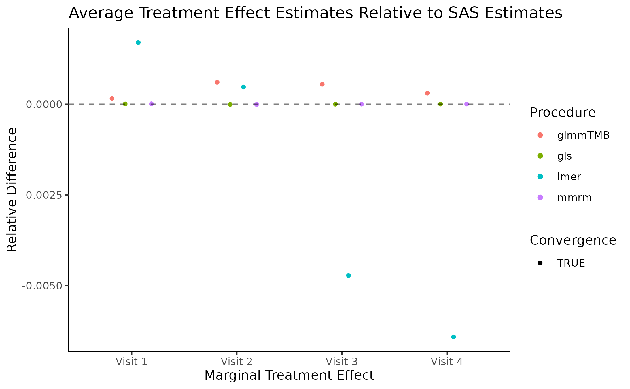
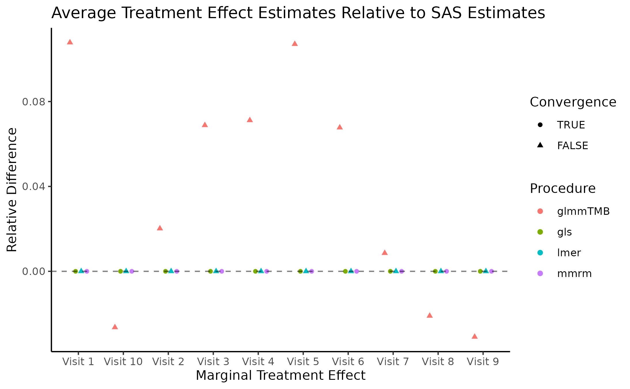
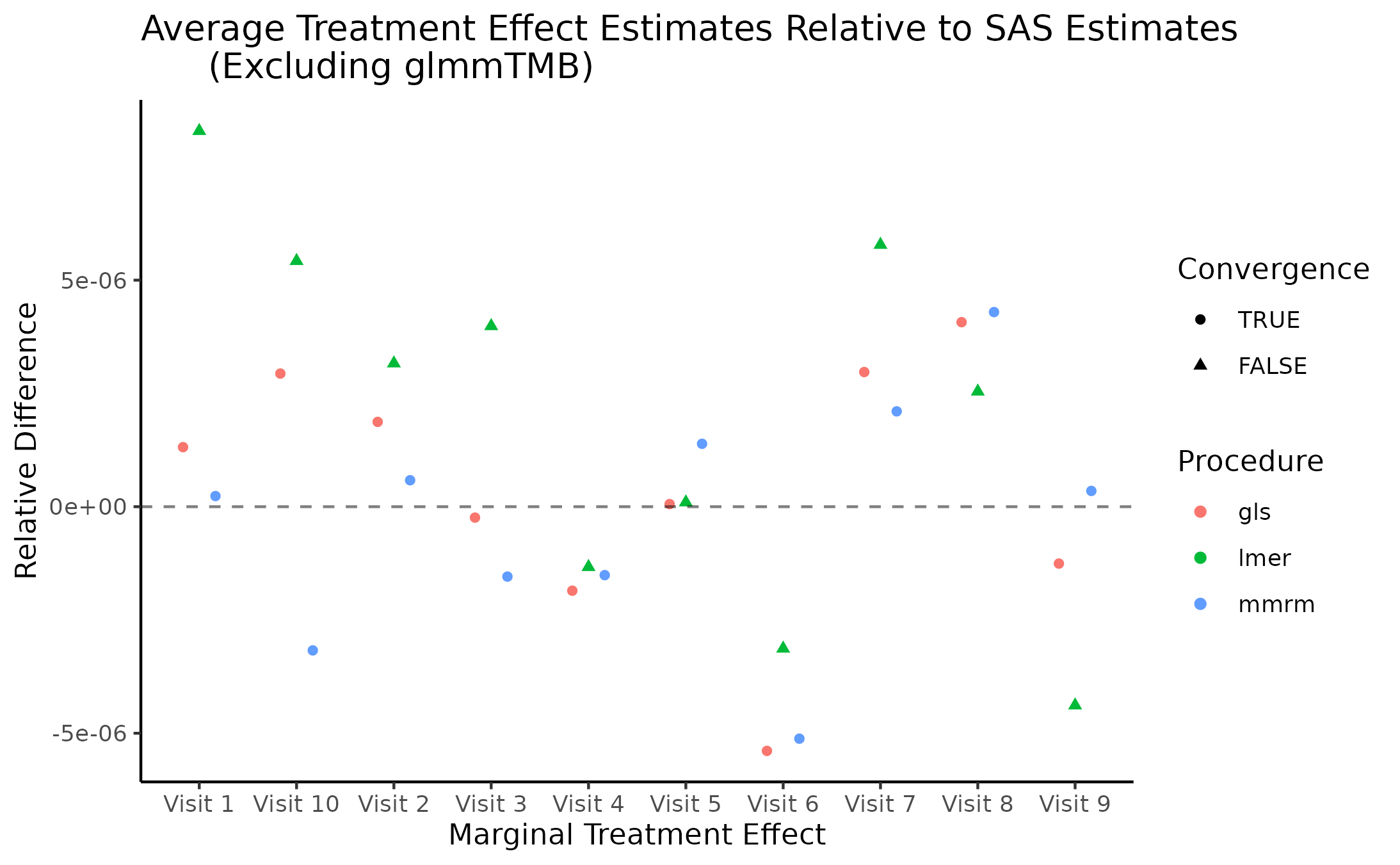
Marginal Treatment Effect Estimates Comparison
We next estimate the marginal mean treatment effects for each visit
in the FEV and BCVA datasets using the MMRM fitting procedures. All R
implementations’ estimates are reported relative to
PROC GLIMMIX’s estimates. Convergence status is also
reported.
Impact of Missing Data on Convergence Rates
The results of the previous benchmark suggest that the amount of patients missing from later time points affect certain implementations’ capacity to converge. We investigate this further by simulating data using a data-generating process similar to that of the BCVA datasets, though with various rates of patient dropout.
Ten datasets of 200 patients are generated each of the following levels of missingness: none, mild, moderate, and high. In all scenarios, observations are missing at random. The number patients observed at each visit is obtained for one replicated dataset at each level of missingness is presented in the table below.
| none | mild | moderate | high | |
|---|---|---|---|---|
| VIS01 | 200 | 196.7 | 197.6 | 188.1 |
| VIS02 | 200 | 195.4 | 194.4 | 182.4 |
| VIS03 | 200 | 195.1 | 190.7 | 175.2 |
| VIS04 | 200 | 194.1 | 188.4 | 162.8 |
| VIS05 | 200 | 191.6 | 182.5 | 142.7 |
| VIS06 | 200 | 188.2 | 177.3 | 125.4 |
| VIS07 | 200 | 184.6 | 168.0 | 105.9 |
| VIS08 | 200 | 178.5 | 155.4 | 82.6 |
| VIS09 | 200 | 175.3 | 139.9 | 58.1 |
| VIS10 | 200 | 164.1 | 124.0 | 39.5 |
The convergence rates of all implementations for stratified by missingness level is presented in the plot below.
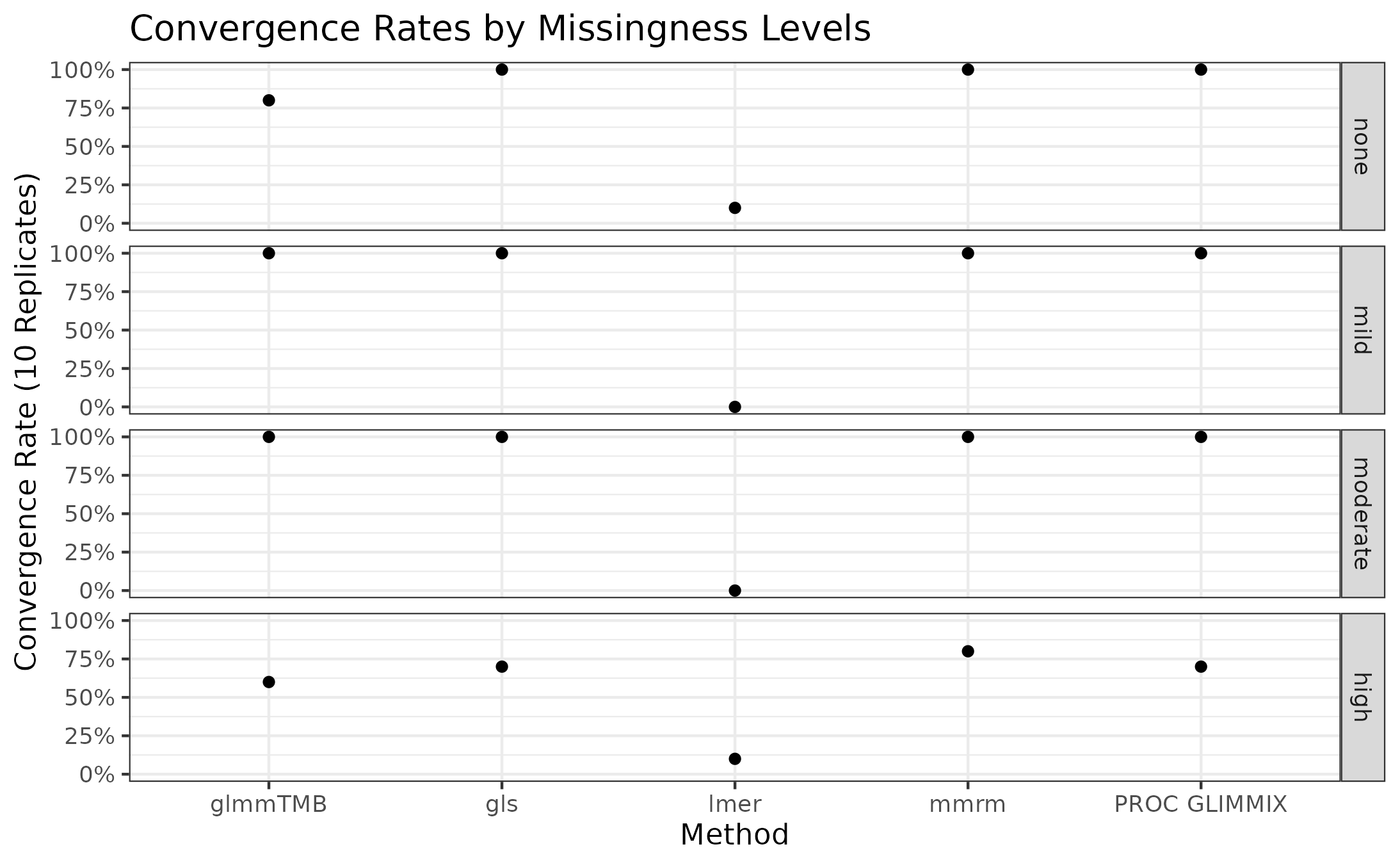
mmrm, gls, and PROC GLIMMIX
are resilient to missingness, only exhibiting some convergence problems
in the scenarios with the most missingness. These implementations
converged in all the other scenarios’ replicates. glmmTMB,
on the other hand, has convergence issues in the no-, mild-, and
high-missingness datasets, with the worst convergence rate occurring in
the datasets with the most dropout. Finally, lmer is
unreliable in all scenarios, suggesting that it’s convergence issues
stem from something other than the missing observations.
Note that the default optimization schemes are used for each method; these schemes can be modified to potentially improve convergence rates.
A more comprehensive simulation study using data-generating processes
similar to the one used here is outlined in the simulations/missing-data-benchmarks
subdirectory. In addition to assessing the effect of missing data on
software convergence rates, we also evaluate these methods’ fit times
and empirical bias, variance, 95% coverage rates, type I error rates and
type II error rates. mmrm is found to be the most most
robust software for fitting MMRMs in scenarios where a large proportion
of patients are missing from the last time points. Additionally,
mmrm has the fastest average fit times regardless of the
amount of missingness. All implementations considered produce similar
empirical biases, variances, 95% coverage rates, type I error rates and
type II error rates.
Session Information
#> R version 4.5.2 (2025-10-31)
#> Platform: x86_64-pc-linux-gnu
#> Running under: Ubuntu 24.04.4 LTS
#>
#> Matrix products: default
#> BLAS:   /usr/lib/x86_64-linux-gnu/openblas-pthread/libblas.so.3
#> LAPACK: /usr/lib/x86_64-linux-gnu/openblas-pthread/libopenblasp-r0.3.26.so;  LAPACK version 3.12.0
#>
#> locale:
#>  [1] LC_CTYPE=en_US.UTF-8       LC_NUMERIC=C
#>  [3] LC_TIME=en_US.UTF-8        LC_COLLATE=en_US.UTF-8
#>  [5] LC_MONETARY=en_US.UTF-8    LC_MESSAGES=en_US.UTF-8
#>  [7] LC_PAPER=en_US.UTF-8       LC_NAME=C
#>  [9] LC_ADDRESS=C               LC_TELEPHONE=C
#> [11] LC_MEASUREMENT=en_US.UTF-8 LC_IDENTIFICATION=C
#>
#> time zone: Etc/UTC
#> tzcode source: system (glibc)
#>
#> attached base packages:
#> [1] stats     graphics  grDevices utils     datasets  methods   base
#>
#> other attached packages:
#>  [1] ggplot2_4.0.3           emmeans_2.0.3           knitr_1.51
#>  [4] sasr_0.1.5              glmmTMB_1.1.14          nlme_3.1-169
#>  [7] lme4_2.0-1              Matrix_1.7-5            mmrm_0.3.18
#> [10] stringr_1.6.0           microbenchmark_1.5.0    purrr_1.2.2
#> [13] dplyr_1.2.1             clusterGeneration_1.3.8 MASS_7.3-65
#>
#> loaded via a namespace (and not attached):
#>  [1] gtable_0.3.6        TMB_1.9.21          xfun_0.59
#>  [4] bslib_0.11.0        htmlwidgets_1.6.4   lattice_0.22-9
#>  [7] numDeriv_2016.8-1.1 vctrs_0.7.3         tools_4.5.2
#> [10] Rdpack_2.6.6        generics_0.1.4      sandwich_3.1-1
#> [13] tibble_3.3.1        pkgconfig_2.0.3     checkmate_2.3.4
#> [16] RColorBrewer_1.1-3  S7_0.2.2            desc_1.4.3
#> [19] lifecycle_1.0.5     farver_2.1.2        compiler_4.5.2
#> [22] textshaping_1.0.5   htmltools_0.5.9     sass_0.4.10
#> [25] yaml_2.3.12         pillar_1.11.1       pkgdown_2.2.0
#> [28] nloptr_2.2.1        jquerylib_0.1.4     cachem_1.1.0
#> [31] reformulas_0.4.4    boot_1.3-32         tidyselect_1.2.1
#> [34] digest_0.6.39       mvtnorm_1.4-1       stringi_1.8.7
#> [37] labeling_0.4.3      splines_4.5.2       fastmap_1.2.0
#> [40] grid_4.5.2          cli_3.6.6           magrittr_2.0.5
#> [43] dichromat_2.0-0.1   withr_3.0.3         scales_1.4.0
#> [46] backports_1.5.1     estimability_2.0.0  rmarkdown_2.31
#> [49] otel_0.2.0          reticulate_1.46.0   ragg_1.5.2
#> [52] zoo_1.8-15          png_0.1-9           coda_0.19-4.1
#> [55] evaluate_1.0.5      rbibutils_2.4.1     mgcv_1.9-4
#> [58] rlang_1.2.0         Rcpp_1.1.1-1.1      xtable_1.8-8
#> [61] glue_1.8.1          minqa_1.2.8         jsonlite_2.0.0
#> [64] R6_2.6.1            systemfonts_1.3.2   fs_2.1.0