Fit dose-response models via bootstrap model averaging (bagging)

This function fits dose-response models in a bootstrap model averaging approach motivated by the bagging procedure (Breiman 1996). Given summary estimates for the outcome at each dose, the function samples summary data from the multivariate normal distribution. For each sample dose-response models are fit to these summary estimates and the best model according to the gAIC is selected.

Usage

maFitMod(dose, resp, S, models, nSim = 1000, control, bnds, addArgs = NULL)

# S3 method for class 'maFit'
predict(
  object,
  summaryFct = function(x) quantile(x, probs = c(0.025, 0.25, 0.5, 0.75, 0.975)),
  doseSeq = NULL,
  ...
)

# S3 method for class 'maFit'
plot(
  x,
  plotData = c("means", "meansCI", "none"),
  xlab = "Dose",
  ylab = "Response",
  title = NULL,
  level = 0.95,
  trafo = function(x) x,
  lenDose = 201,
  ...
)

Arguments

dose: Numeric specifying the dose variable.
resp: Numeric specifying the response estimate corresponding to the doses in dose
S: Covariance matrix associated with the dose-response estimate specified via resp
models: dose-response models to fit
nSim: Number of bootstrap simulations
control: Same as the control argument in fitMod.
bnds: Bounds for non-linear parameters. This needs to be a list with list entries corresponding to the selected bounds. The names of the list entries need to correspond to the model names. The defBnds function provides the default selection.
addArgs: List containing two entries named "scal" and "off" for the "betaMod" and "linlog" model. When addArgs is NULL the following defaults are used list(scal = 1.2*max(doses), off = 0.01*max(doses))
object: Object of class maFit
summaryFct: If equal to NULL predictions are calculated for each sampled parameter value. Otherwise a summary function is applied to the dose-response predictions for each parameter value. The default is to calculate 0.025, 0.25, 0.5, 0.75, 0.975 quantiles of the predictions for each dose.
doseSeq: Where to calculate predictions.
...: Additional parametes (unused)
x: object of class maFit
plotData: Determines how the original data are plotted: Either as means or as means with CI or not at all. The level of the CI is determined by the argument level.
xlab: x-axis label
ylab: y-axis label
title: plot title
level: Level for CI, when plotData is equal to meansCI.
trafo: Plot the fitted models on a transformed scale (e.g. probability scale if models have been fitted on log-odds scale). The default for trafo is the identity function.
lenDose: Number of grid values to use for display.

Value

An object of class maFit, which contains the fitted dose-response models DRMod objects, information on which model was selected in each bootstrap and basic input parameters.

References

Breiman, L. (1996). Bagging predictors. Machine learning, 24, 123-140.

Author

Bjoern Bornkamp

Examples

data(biom)
## produce first stage fit (using dose as factor)
anMod <- lm(resp~factor(dose)-1, data=biom)
drFit <- coef(anMod)
S <- vcov(anMod)
dose <- sort(unique(biom$dose))
## fit an emax and sigEmax model (increase nSim for real use)
mFit <- maFitMod(dose, drFit, S, model = c("emax", "sigEmax"), nSim = 10)
#> Message: Need bounds in "bnds" for nonlinear models, using default bounds from "defBnds".
mFit
#> Bootstrap model averaging fits
#> 
#> Specified summary data:
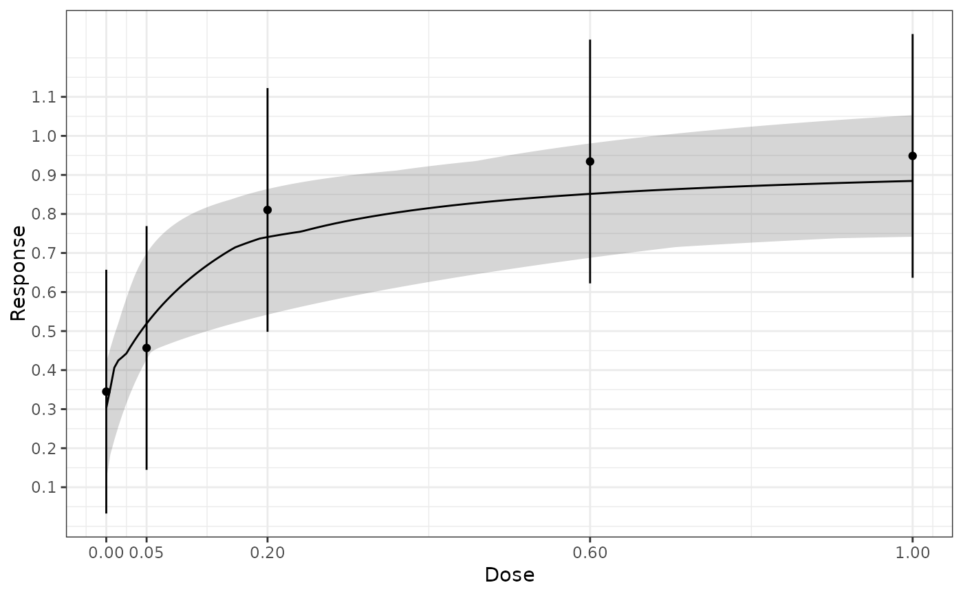
#> doses: 0, 0.05, 0.2, 0.6, 1
#> mean: 0.345, 0.457, 0.81, 0.934, 0.949
#> Covariance Matrix:
#>          0  0.05   0.2   0.6     1
#> 0    0.025 0.000 0.000 0.000 0.000
#> 0.05 0.000 0.025 0.000 0.000 0.000
#> 0.2  0.000 0.000 0.025 0.000 0.000
#> 0.6  0.000 0.000 0.000 0.025 0.000
#> 1    0.000 0.000 0.000 0.000 0.025
#> 
#> Models fitted: emax, sigEmax
#> 
#> Models selected by gAIC on bootstrap samples (nSim = 10)
#> emax 
#>   10 
plot(mFit, plotData = "meansCI")

ED(mFit, direction = "increasing", p = 0.9)
#> [1] 0.45

References

Breiman L (1996). “Baggin predictors.” Machine Learning, 24(2), 123-140. doi:10.1007/bf00058655 .