Usage

This vignette explains how to use the pmrm package

Raw data

The package functions expect tidy longitudinal data with one row per subject visit and columns with the patient outcome, continuous time, indicator variables, and optional covariates. The pmrm package has functions to simulate datasets from each supported model.

library(pmrm)
set.seed(0)
simulation <- pmrm_simulate_decline_proportional(
  patients = 500,
  visit_times = c(0, 1, 2, 3, 4),
  tau = 0.25,
  alpha = c(0, 0.7, 1, 1.4, 1.6),
  beta = c(0, 0.2, 0.35),
  gamma = c(-1, 1)
)

The outcome column can have missing values, but no other column must have missing values.¹

simulation$y[c(2L, 3L, 12L, 13L, 14L, 15L)] <- NA_real_

The output datasets includes important information that you would supply to a modeling function.

simulation[, c("y", "t", "patient", "visit", "arm")]
#> # A tibble: 2,500 × 5
#>         y     t patient   visit   arm  
#>     <dbl> <dbl> <chr>     <ord>   <ord>
#>  1  2.20   0    patient_1 visit_1 arm_1
#>  2 NA      1.47 patient_1 visit_2 arm_1
#>  3 NA      1.90 patient_1 visit_3 arm_1
#>  4  1.93   2.73 patient_1 visit_4 arm_1
#>  5  3.33   4.04 patient_1 visit_5 arm_1
#>  6 -4.75   0    patient_2 visit_1 arm_2
#>  7  0.271  1.16 patient_2 visit_2 arm_2
#>  8  1.95   1.97 patient_2 visit_3 arm_2
#>  9  1.99   3.09 patient_2 visit_4 arm_2
#> 10  3.60   4.45 patient_2 visit_5 arm_2
#> # ℹ 2,490 more rows

Models

To fit a model, simply supply the preprocessed dataset and optionally the knot vector xi (which usually just contains the scheduled times of all the visits). The package is powered by the RTMB package, so the model fitting process runs fast.

system.time(
  fit <- pmrm_model_decline_proportional(
    data = simulation,
    outcome = "y",
    time = "t",
    patient = "patient",
    visit = "visit",
    arm = "arm",
    covariates = ~ w_1 + w_2,
    visit_times = c(0, 1, 2, 3, 4)
  )
)
#>    user  system elapsed 
#>   0.447   0.011   0.458

print(fit)
#> Model:
#> 
#>   PMRM type:        decline
#>   Parameterization: proportional
#> 
#> Fit:
#> 
#>   Convergence:    converged
#>   Observations:   2494
#>   Parameters:     24
#>   Log likelihood: -3555.535
#>   Deviance:       7111.071
#>   AIC:            7159.071
#>   BIC:            7298.79
#> 
#> Treatment effects:
#> 
#>          estimate  std.error
#>   arm_2 0.2493296 0.04117794
#>   arm_3 0.3749138 0.04023259

The fitted model object has parameter estimates, standard errors, model constants, the convergence status, raw RTMB objects, and other information.

names(fit)
#>  [1] "data"            "constants"       "options"         "objective"      
#>  [5] "model"           "optimization"    "report"          "initial"        
#>  [9] "final"           "estimates"       "standard_errors" "metrics"        
#> [13] "spline"

All estimates:²

str(fit$estimates)
#> List of 9
#>  $ alpha : Named num [1:5] 0.0269 0.763 0.9555 1.4059 1.6247
#>   ..- attr(*, "names")= chr [1:5] "1" "2" "3" "4" ...
#>  $ theta : num [1:2] 0.249 0.375
#>  $ gamma : num [1:2] -0.954 0.995
#>  $ phi   : num [1:5] 0.0364 0.0134 -0.0022 -0.0399 0.0403
#>  $ rho   : num [1:10] -0.0429 -0.0824 0.0437 -0.0715 -0.0532 ...
#>  $ beta  : num [1:3] 0 0.249 0.375
#>  $ sigma : num [1:5] 1.037 1.014 0.998 0.961 1.041
#>  $ Lambda: num [1:5, 1:5] 1 -0.0428 -0.082 0.0436 -0.0712 ...
#>  $ Sigma : num [1:5, 1:5] 1.0756 -0.045 -0.0849 0.0434 -0.0768 ...

Just the estimates of actual parameters, omitting functions of other parameters:³

str(fit$final)
#> List of 5
#>  $ alpha: Named num [1:5] 0.0269 0.763 0.9555 1.4059 1.6247
#>   ..- attr(*, "names")= chr [1:5] "1" "2" "3" "4" ...
#>  $ theta: num [1:2] 0.249 0.375
#>  $ gamma: num [1:2] -0.954 0.995
#>  $ phi  : num [1:5] 0.0364 0.0134 -0.0022 -0.0399 0.0403
#>  $ rho  : num [1:10] -0.0429 -0.0824 0.0437 -0.0715 -0.0532 ...

Checking and troubleshooting

Model-checking is an involved topic, and pmrm itself does not go into tremendous depth. Instead, it offers only the most basic checks on the fitted model object. The goal is to guide your intuition and high-level understanding.

First, check the convergence code. A 0 indicates convergence, and a 1 indicates that the model diverged or a local minimum was not otherwise reached (e.g. in the case of a saddle point).

fit$optimization$convergence
#> [1] 0

Next, you may wish to check that the parameter estimates and standard errors make sense.

str(fit$estimates)
#> List of 9
#>  $ alpha : Named num [1:5] 0.0269 0.763 0.9555 1.4059 1.6247
#>   ..- attr(*, "names")= chr [1:5] "1" "2" "3" "4" ...
#>  $ theta : num [1:2] 0.249 0.375
#>  $ gamma : num [1:2] -0.954 0.995
#>  $ phi   : num [1:5] 0.0364 0.0134 -0.0022 -0.0399 0.0403
#>  $ rho   : num [1:10] -0.0429 -0.0824 0.0437 -0.0715 -0.0532 ...
#>  $ beta  : num [1:3] 0 0.249 0.375
#>  $ sigma : num [1:5] 1.037 1.014 0.998 0.961 1.041
#>  $ Lambda: num [1:5, 1:5] 1 -0.0428 -0.082 0.0436 -0.0712 ...
#>  $ Sigma : num [1:5, 1:5] 1.0756 -0.045 -0.0849 0.0434 -0.0768 ...

str(fit$standard_errors)
#> List of 9
#>  $ alpha : Named num [1:5] 0.0455 0.0637 0.0609 0.063 0.0636
#>   ..- attr(*, "names")= chr [1:5] "1" "2" "3" "4" ...
#>  $ theta : num [1:2] 0.0412 0.0402
#>  $ gamma : num [1:2] 0.0206 0.0205
#>  $ phi   : num [1:5] 0.0316 0.0317 0.0318 0.0318 0.0318
#>  $ rho   : num [1:10] 0.0449 0.0451 0.0449 0.0451 0.0449 ...
#>  $ beta  : num [1:3] 0 0.0412 0.0402
#>  $ sigma : num [1:5] 0.0328 0.0321 0.0318 0.0306 0.0331
#>  $ Lambda: num [1:5, 1:5] 0 0.0447 0.0446 0.0447 0.0446 ...
#>  $ Sigma : num [1:5, 1:5] 0.0681 0.0472 0.0466 0.0447 0.0486 ...

Also, please check for odd behavior in the fitted spline $f(x | \xi, \alpha)$.

knots <- fit$constants$spline_knots
curve(fit$spline(x), min(knots), max(knots))

In tough cases, the spline may flatten out at the knot boundaries or twist in strange directions. If you notice a strange fitted spline in a divergent model, you may wish to experiment with different knot placement or hand-pick initial values for the vertical knot distances alpha. The latter can sometimes help stabilize theta (especially for pmrm_model_slowing()) by beginning with an appropriately strict monotone spline. Example:

initial <- fit$initial
initial$alpha <- c(0, 0.5, 1, 1.5, 2)

fit2 <- pmrm_model_decline_proportional(
  data = simulation,
  outcome = "y",
  time = "t",
  patient = "patient",
  visit = "visit",
  arm = "arm",
  covariates = ~ w_1 + w_2,
  visit_times = c(0, 1, 2, 3, 4),
  initial = initial # with hand-picked initial alpha
)

Alternatively, you can even tweak one or more parameters and then resume the original optimization.

initial <- fit$final # true parameters from the last fit
initial$theta[2] <- 0 # reset a scalar parameter that may have diverged

fit3 <- pmrm_model_decline_proportional(
  data = simulation,
  outcome = "y",
  time = "t",
  patient = "patient",
  visit = "visit",
  arm = "arm",
  covariates = ~ w_1 + w_2,
  visit_times = c(0, 1, 2, 3, 4),
  initial = initial # with the modified parameter values
)

Finally, you may wish to fit a Bayesian version the model using tmbstan and check for correlations among the parameters. Strong pairwise correlations involving the $\alpha$ parameter may indicate that your spline has too many knots.

library(dplyr)
library(tmbstan)
library(posterior)

# Fit a Bayesian version of the same model.
# Increase the number of chains for the Rhat diagnostic to be valid.
mcmc <- tmbstan(fit$model, chains = 1, refresh = 10)

# Extract the MCMC draws.
draws <- as_draws_df(mcmc) |>
  select(starts_with("alpha"), any_of(c("theta", "phi")))

# Plot pairwise correlations among MCMC draws.
# Pairs of parameters should not be strongly correlated.
# Tight correlations and funneling indicate problems,
# such as non-identifiability if you have too many knots.
pairs(draws)

# Alternatively, if you have many parameters, you can look at
# pairwise linear correlations. However, this may miss
# important pathologies.
correlations <- cor(samples)[lower.tri(cor(samples))]
hist(correlations)

Summaries

Use pmrm_estimates() to compute estimates, standard errors, and confidence intervals of model parameters and standard downstream functions of parameters. For example, here are the active-arm post-baseline treatment effect parameters:

pmrm_estimates(fit, parameter = "theta")
#> # A tibble: 2 × 6
#>   parameter arm   estimate standard_error lower upper
#>   <chr>     <ord>    <dbl>          <dbl> <dbl> <dbl>
#> 1 theta     arm_2    0.249         0.0412 0.169 0.330
#> 2 theta     arm_3    0.375         0.0402 0.296 0.454

And the same for the visit-specific standard deviations of the residuals:

pmrm_estimates(fit, parameter = "sigma", confidence = 0.9)
#> # A tibble: 5 × 6
#>   parameter visit   estimate standard_error lower upper
#>   <chr>     <ord>      <dbl>          <dbl> <dbl> <dbl>
#> 1 sigma     visit_1    1.04          0.0328 0.983  1.09
#> 2 sigma     visit_2    1.01          0.0321 0.961  1.07
#> 3 sigma     visit_3    0.998         0.0318 0.946  1.05
#> 4 sigma     visit_4    0.961         0.0306 0.911  1.01
#> 5 sigma     visit_5    1.04          0.0331 0.987  1.10

The summary() method produces high-level metrics for model comparison.

summary(fit)
#> # A tibble: 1 × 8
#>   model   parameterization n_observations n_parameters log_likelihood deviance
#>   <chr>   <chr>                     <int>        <int>          <dbl>    <dbl>
#> 1 decline proportional               2494           24         -3556.    7111.
#> # ℹ 2 more variables: aic <dbl>, bic <dbl>

Marginals

pmrm_marginals() returns estimated marginal means for each study arm and visit. The continuous time at each visit is given by the marginals argument to pmrm_model_decline_proportional().

pmrm_marginals(fit, type = "outcome")
#> # A tibble: 15 × 7
#>    arm   visit    time estimate standard_error   lower upper
#>    <ord> <ord>   <dbl>    <dbl>          <dbl>   <dbl> <dbl>
#>  1 arm_1 visit_1     0   0.0269         0.0455 -0.0623 0.116
#>  2 arm_1 visit_2     1   0.763          0.0637  0.638  0.888
#>  3 arm_1 visit_3     2   0.955          0.0609  0.836  1.07 
#>  4 arm_1 visit_4     3   1.41           0.0630  1.28   1.53 
#>  5 arm_1 visit_5     4   1.62           0.0636  1.50   1.75 
#>  6 arm_2 visit_1     0   0.0269         0.0455 -0.0623 0.116
#>  7 arm_2 visit_2     1   0.579          0.0497  0.482  0.677
#>  8 arm_2 visit_3     2   0.724          0.0509  0.624  0.824
#>  9 arm_2 visit_4     3   1.06           0.0531  0.958  1.17 
#> 10 arm_2 visit_5     4   1.23           0.0589  1.11   1.34 
#> 11 arm_3 visit_1     0   0.0269         0.0455 -0.0623 0.116
#> 12 arm_3 visit_2     1   0.487          0.0432  0.402  0.572
#> 13 arm_3 visit_3     2   0.607          0.0453  0.518  0.696
#> 14 arm_3 visit_4     3   0.889          0.0511  0.789  0.989
#> 15 arm_3 visit_5     4   1.03           0.0569  0.914  1.14

Select type = "change" for estimates of change from baseline.

pmrm_marginals(fit, type = "change")
#> # A tibble: 15 × 7
#>    arm   visit    time estimate standard_error  lower  upper
#>    <ord> <ord>   <dbl>    <dbl>          <dbl>  <dbl>  <dbl>
#>  1 arm_1 visit_1     0   NA            NA      NA     NA    
#>  2 arm_1 visit_2     1    0.736         0.0825  0.574  0.898
#>  3 arm_1 visit_3     2    0.929         0.0793  0.773  1.08 
#>  4 arm_1 visit_4     3    1.38          0.0757  1.23   1.53 
#>  5 arm_1 visit_5     4    1.60          0.0782  1.44   1.75 
#>  6 arm_2 visit_1     0   NA            NA      NA     NA    
#>  7 arm_2 visit_2     1    0.553         0.0684  0.419  0.687
#>  8 arm_2 visit_3     2    0.697         0.0696  0.561  0.833
#>  9 arm_2 visit_4     3    1.04          0.0697  0.899  1.17 
#> 10 arm_2 visit_5     4    1.20          0.0770  1.05   1.35 
#> 11 arm_3 visit_1     0   NA            NA      NA     NA    
#> 12 arm_3 visit_2     1    0.460         0.0612  0.340  0.580
#> 13 arm_3 visit_3     2    0.580         0.0639  0.455  0.706
#> 14 arm_3 visit_4     3    0.862         0.0685  0.728  0.996
#> 15 arm_3 visit_5     4    0.999         0.0762  0.849  1.15

Select type = "effect" for estimates of the treatment effect (change from baseline of each active arm minus that of the control arm).

pmrm_marginals(fit, type = "effect")
#> # A tibble: 15 × 7
#>    arm   visit    time estimate standard_error  lower  upper
#>    <ord> <ord>   <dbl>    <dbl>          <dbl>  <dbl>  <dbl>
#>  1 arm_1 visit_1     0   NA            NA      NA     NA    
#>  2 arm_1 visit_2     1   NA            NA      NA     NA    
#>  3 arm_1 visit_3     2   NA            NA      NA     NA    
#>  4 arm_1 visit_4     3   NA            NA      NA     NA    
#>  5 arm_1 visit_5     4   NA            NA      NA     NA    
#>  6 arm_2 visit_1     0   NA            NA      NA     NA    
#>  7 arm_2 visit_2     1   -0.184         0.0370 -0.256 -0.111
#>  8 arm_2 visit_3     2   -0.232         0.0437 -0.317 -0.146
#>  9 arm_2 visit_4     3   -0.344         0.0641 -0.469 -0.218
#> 10 arm_2 visit_5     4   -0.398         0.0729 -0.541 -0.255
#> 11 arm_3 visit_1     0   NA            NA      NA     NA    
#> 12 arm_3 visit_2     1   -0.276         0.0413 -0.357 -0.195
#> 13 arm_3 visit_3     2   -0.348         0.0463 -0.439 -0.257
#> 14 arm_3 visit_4     3   -0.517         0.0652 -0.645 -0.389
#> 15 arm_3 visit_5     4   -0.599         0.0736 -0.743 -0.455

Predictions

The package supports a predict() method for all PMRMs. It returns the expected values, standard errors, and confidence intervals for the outcomes given new data. All the important columns from the original data need to be part of the new data, except that the outcome column can be entirely absent.

predict(fit, data = head(simulation, 5))
#> # A tibble: 5 × 7
#>   arm   visit    time estimate standard_error  lower  upper
#>   <ord> <ord>   <dbl>    <dbl>          <dbl>  <dbl>  <dbl>
#> 1 arm_1 visit_1  0       0.939         0.0476  0.846  1.03 
#> 2 arm_1 visit_2  1.47    1.69          0.0521  1.59   1.80 
#> 3 arm_1 visit_3  1.90   -1.39          0.0697 -1.52  -1.25 
#> 4 arm_1 visit_4  2.73    0.622         0.0609  0.503  0.742
#> 5 arm_1 visit_5  4.04    2.92          0.0690  2.79   3.06

Plots

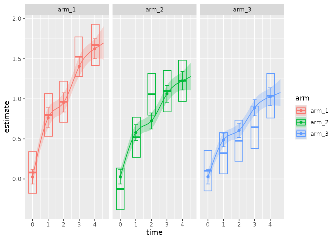
pmrm supports an S3 method for the plot() generic. This method plot.pmrm_fit() visually compares the model to the data. The default plot shows:

• Raw estimates and confidence intervals on the data, as points and vertical line segments.
• Model-based marginal means and confidence intervals, as horizontal line segments and boxes around them.
• Model-based predictions and confidence bands, as continuous lines and shaded regions.

plot(
  fit,
  show_predictions = TRUE # Defaults to FALSE because predictions take extra time.
)

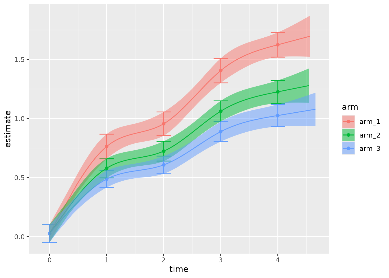
You can customize the plot: for example, to compare the fitted disease progression trajectory across treatment arms.

plot(
  fit,
  confidence = 0.9,
  show_data = FALSE,
  show_predictions = TRUE, # Defaults to FALSE because predictions take extra time.
  facet = FALSE,
  alpha = 0.5
)