Introduction
Clinical trial analyses that use reference-based multiple imputation
typically involve several steps: fitting an imputation model, generating
imputed datasets, applying an analysis to each dataset, and pooling
results using Rubin’s rules. The rbmi package
implements this pipeline with its draws(),
impute(), analyse(), and pool()
functions. However, turning the pooled results into publication-ready
outputs – formatted tables and forest plots suitable for regulatory
submissions – requires additional work.
The rbmiUtils package bridges this gap. It provides utilities that sit on top of rbmi, transforming pooled analysis objects into tidy data frames, regulatory-style efficacy tables, and three-panel forest plots. It also includes data preparation helpers that catch common issues before the computationally expensive imputation step.
In this vignette, you will walk through the complete pipeline from raw clinical trial data to two publication-ready outputs: an efficacy summary table and a forest plot. By the end, you will have seen every major step in a typical rbmi + rbmiUtils workflow. For a more focused reference on the analysis functions, see the analyse2 vignette. For detailed guidance on data preparation, see the data preparation vignette.
Setup and Data
We begin by loading the packages we need. The core pipeline requires rbmi and rbmiUtils, with dplyr for data manipulation. The reporting outputs use gt (for tables) and ggplot2 + patchwork (for plots), which are optional dependencies.
The ADEFF dataset bundled with rbmiUtils is a simulated
ADaM-style efficacy dataset from a two-arm clinical trial. It contains
continuous change-from-baseline outcomes (CHG) measured at
two visits (Week 24 and Week 48), with realistic missing data patterns
across 500 subjects.
data("ADEFF", package = "rbmiUtils")
str(ADEFF)
#> tibble [1,000 × 10] (S3: tbl_df/tbl/data.frame)
#>  $ USUBJID: chr [1:1000] "ID001" "ID001" "ID002" "ID002" ...
#>   ..- attr(*, "label")= chr "Unique patient identifier"
#>  $ STRATA : chr [1:1000] "A" "A" "A" "A" ...
#>   ..- attr(*, "label")= chr "Stratification at randomisation"
#>  $ REGION : chr [1:1000] "North America" "North America" "Asia" "Asia" ...
#>   ..- attr(*, "label")= chr "Stratification by region"
#>  $ REGIONC: num [1:1000] 1 1 4 4 2 2 3 3 2 2 ...
#>   ..- attr(*, "label")= chr "Stratification by region, numeric code"
#>  $ TRT01P : chr [1:1000] "Drug A" "Drug A" "Drug A" "Drug A" ...
#>   ..- attr(*, "label")= chr "Planned treatment"
#>  $ BASE   : num [1:1000] 16 16 10 10 12 12 11 11 9 9 ...
#>   ..- attr(*, "label")= chr "Baseline value of primary outcome variable"
#>  $ AVISIT : chr [1:1000] "Week 24" "Week 48" "Week 24" "Week 48" ...
#>   ..- attr(*, "label")= chr "Visit number"
#>  $ AVAL   : num [1:1000] 12 13 7 5 9 10 9 13 4 0 ...
#>   ..- attr(*, "label")= chr "Primary outcome variable"
#>  $ PARAM  : chr [1:1000] "ESSDAI score" "ESSDAI score" "ESSDAI score" "ESSDAI score" ...
#>   ..- attr(*, "label")= chr "Analysis parameter name"
#>  $ CHG    : num [1:1000] -4 -3 -3 -5 -3 -2 -2 2 -5 -9 ...
#>   ..- attr(*, "label")= chr "Change from baseline"
Before entering the rbmi pipeline, we convert the key grouping columns to factors. Factor levels control the ordering of treatment arms and visits throughout the analysis, so it is important to set them explicitly.
Data Preparation
Before running the imputation model, it is worth investing a moment
to validate the data and understand the missing data patterns. These
checks can save considerable time by catching issues before the
computationally intensive draws() step.
Validation
The validate_data() function performs a comprehensive
set of pre-flight checks: it verifies that all required columns exist,
that factors are properly typed, that the outcome is numeric, that
covariates have no missing values, and that there are no duplicate
subject-visit rows.
vars <- set_vars(
  subjid = "USUBJID",
  visit = "AVISIT",
  group = "TRT",
  outcome = "CHG",
  covariates = c("BASE", "STRATA", "REGION")
)
validate_data(ADEFF, vars)A successful validation returns TRUE silently. If issues
are found, all problems are reported together in a single error message
so you can fix them in one pass.
Missingness Summary
The summarise_missingness() function characterises the
missing data patterns in your dataset, classifying each subject as
complete, monotone (dropout), or intermittent.
miss <- summarise_missingness(ADEFF, vars)
print(miss$summary)
#> # A tibble: 2 × 5
#>   group   n_subjects n_complete n_monotone n_intermittent
#>   <chr>        <int>      <int>      <int>          <int>
#> 1 Drug A         261        239         11             11
#> 2 Placebo        239        217         16              6
This summary helps you decide on an appropriate imputation strategy.
For datasets that require intercurrent event (ICE) handling, rbmiUtils
also provides prepare_data_ice() to build the
data_ice data frame from flag columns – see the data preparation vignette for
details.
rbmi Analysis Pipeline
With the data validated, we now run the core rbmi pipeline. This consists of four steps: specifying the imputation method, fitting the imputation model, generating imputed datasets, and analysing each one.
Specify the Imputation Method
The method_bayes() function configures Bayesian multiple
imputation using MCMC sampling. Here we use a small number of samples
and a short warmup period to keep the vignette build time manageable. In
a real analysis, you would typically use more samples (e.g.,
n_samples = 500 or more) for better precision. For details
on the statistical methodology, see the rbmi
quickstart vignette.
set.seed(1974)

method <- method_bayes(
  n_samples = 100,
  control = control_bayes(warmup = 200, thin = 2)
)
Fit the Imputation Model
The draws() function fits the Bayesian imputation model.
This is the most computationally intensive step in the pipeline. We pass
the dataset with only the columns needed for the model.
dat <- ADEFF |>
  select(USUBJID, STRATA, REGION, TRT, BASE, CHG, AVISIT)

draws_obj <- draws(data = dat, vars = vars, method = method)
#> Running /opt/R/4.5.2/lib/R/bin/R CMD SHLIB foo.c
#> using C compiler: ‘gcc (Ubuntu 13.3.0-6ubuntu2~24.04) 13.3.0’
#> gcc -std=gnu2x -I"/opt/R/4.5.2/lib/R/include" -DNDEBUG   -I"/home/runner/work/_temp/Library/Rcpp/include/"  -I"/home/runner/work/_temp/Library/RcppEigen/include/"  -I"/home/runner/work/_temp/Library/RcppEigen/include/unsupported"  -I"/home/runner/work/_temp/Library/BH/include" -I"/home/runner/work/_temp/Library/StanHeaders/include/src/"  -I"/home/runner/work/_temp/Library/StanHeaders/include/"  -I"/home/runner/work/_temp/Library/RcppParallel/include/"  -I"/home/runner/work/_temp/Library/rstan/include" -DEIGEN_NO_DEBUG  -DBOOST_DISABLE_ASSERTS  -DBOOST_PENDING_INTEGER_LOG2_HPP  -DSTAN_THREADS  -DUSE_STANC3 -DSTRICT_R_HEADERS  -DBOOST_PHOENIX_NO_VARIADIC_EXPRESSION  -D_HAS_AUTO_PTR_ETC=0  -include '/home/runner/work/_temp/Library/StanHeaders/include/stan/math/prim/fun/Eigen.hpp'  -D_REENTRANT -DRCPP_PARALLEL_USE_TBB=1   -I/usr/local/include    -fpic  -g -O2  -c foo.c -o foo.o
#> In file included from /home/runner/work/_temp/Library/RcppEigen/include/Eigen/Core:19,
#>                  from /home/runner/work/_temp/Library/RcppEigen/include/Eigen/Dense:1,
#>                  from /home/runner/work/_temp/Library/StanHeaders/include/stan/math/prim/fun/Eigen.hpp:22,
#>                  from <command-line>:
#> /home/runner/work/_temp/Library/RcppEigen/include/Eigen/src/Core/util/Macros.h:679:10: fatal error: cmath: No such file or directory
#>   679 | #include <cmath>
#>       |          ^~~~~~~
#> compilation terminated.
#> make: *** [/opt/R/4.5.2/lib/R/etc/Makeconf:202: foo.o] Error 1
#>
#> SAMPLING FOR MODEL 'rbmi_MMRM_us_default' NOW (CHAIN 1).
#> Chain 1:
#> Chain 1: Gradient evaluation took 0.000473 seconds
#> Chain 1: 1000 transitions using 10 leapfrog steps per transition would take 4.73 seconds.
#> Chain 1: Adjust your expectations accordingly!
#> Chain 1:
#> Chain 1:
#> Chain 1: Iteration:   1 / 400 [  0%]  (Warmup)
#> Chain 1: Iteration:  40 / 400 [ 10%]  (Warmup)
#> Chain 1: Iteration:  80 / 400 [ 20%]  (Warmup)
#> Chain 1: Iteration: 120 / 400 [ 30%]  (Warmup)
#> Chain 1: Iteration: 160 / 400 [ 40%]  (Warmup)
#> Chain 1: Iteration: 200 / 400 [ 50%]  (Warmup)
#> Chain 1: Iteration: 201 / 400 [ 50%]  (Sampling)
#> Chain 1: Iteration: 240 / 400 [ 60%]  (Sampling)
#> Chain 1: Iteration: 280 / 400 [ 70%]  (Sampling)
#> Chain 1: Iteration: 320 / 400 [ 80%]  (Sampling)
#> Chain 1: Iteration: 360 / 400 [ 90%]  (Sampling)
#> Chain 1: Iteration: 400 / 400 [100%]  (Sampling)
#> Chain 1:
#> Chain 1:  Elapsed Time: 0.65 seconds (Warm-up)
#> Chain 1:                0.533 seconds (Sampling)
#> Chain 1:                1.183 seconds (Total)
#> Chain 1:
Generate Imputed Datasets
The impute() function generates complete datasets under
the specified reference-based assumption. Here we use a
jump-to-reference approach where both arms are imputed under the
reference (Placebo) distribution.
Analyse Each Imputed Dataset
Rather than calling rbmi::analyse() directly, rbmiUtils
provides analyse_mi_data(), which wraps the analyse step to
work with the stacked imputed data format. It applies an analysis
function – here, the built-in ancova function – to each
imputed dataset and stores the results for pooling.
First, we extract the imputed data into a stacked data frame using
get_imputed_data():
ADMI <- get_imputed_data(impute_obj)Then we analyse:
ana_obj <- analyse_mi_data(
  data = ADMI,
  vars = vars,
  method = method,
  fun = ancova
)
Pool Results
Finally, pool() combines the per-imputation results
using Rubin’s
rules to produce a single set of estimates, standard errors,
confidence intervals, and p-values.
pool_obj <- pool(ana_obj)
print(pool_obj)
#>        parameter   visit   est   lci   uci    pval
#>      trt_Week 24 Week 24 -2.18 -2.54 -1.82 < 0.001
#>  lsm_ref_Week 24 Week 24  0.08 -0.18  0.33   0.559
#>  lsm_alt_Week 24 Week 24 -2.10 -2.35 -1.85 < 0.001
#>      trt_Week 48 Week 48 -3.81 -4.31 -3.30 < 0.001
#>  lsm_ref_Week 48 Week 48  0.04 -0.32  0.41   0.812
#>  lsm_alt_Week 48 Week 48 -3.76 -4.11 -3.42 < 0.001
Tidying Results
The pool object contains all the information we need, but its
structure is not immediately convenient for reporting. The
tidy_pool_obj() function converts it into a tidy tibble
with clearly labelled columns.
tidy_df <- tidy_pool_obj(pool_obj)
print(tidy_df)
#> # A tibble: 6 × 10
#>   parameter       description visit parameter_type lsm_type     est    se    lci
#>   <chr>           <chr>       <chr> <chr>          <chr>      <dbl> <dbl>  <dbl>
#> 1 trt_Week 24     Treatment … Week… trt            NA       -2.18   0.182 -2.54
#> 2 lsm_ref_Week 24 Least Squa… Week… lsm            ref       0.0765 0.131 -0.181
#> 3 lsm_alt_Week 24 Least Squa… Week… lsm            alt      -2.10   0.126 -2.35
#> 4 trt_Week 48     Treatment … Week… trt            NA       -3.81   0.256 -4.31
#> 5 lsm_ref_Week 48 Least Squa… Week… lsm            ref       0.0440 0.185 -0.320
#> 6 lsm_alt_Week 48 Least Squa… Week… lsm            alt      -3.76   0.175 -4.11
#> # ℹ 2 more variables: uci <dbl>, pval <dbl>
Each row represents one parameter at one visit. The key columns are:
- parameter: the raw parameter name from the pool object
-
parameter_type:
"trt"for treatment differences,"lsm"for least squares means -
lsm_type:
"ref"or"alt"for LS mean rows - visit: the visit name
- est, se, lci, uci, pval: the numeric results
This tidy format is the foundation for all downstream reporting. You can filter, reshape, or format it as needed for your specific tables.
Efficacy Table
The efficacy_table() function takes the pool object and
produces a regulatory-style gt table in the format commonly seen in
ICH/CDISC Table 14.2.x submissions. It displays LS means by arm,
treatment differences, confidence intervals, and p-values, organised by
visit.
tbl <- efficacy_table(pool_obj)
tbl| Estimate | Std. Error | 95% CI | P-value | |
|---|---|---|---|---|
| Week 24 | ||||
| LS Mean (Reference) | 0.08 | 0.13 | (-0.18, 0.33) | 0.559 |
| LS Mean (Treatment) | −2.10 | 0.13 | (-2.35, -1.85) | < 0.001 |
| Treatment Difference | −2.18 | 0.18 | (-2.54, -1.82) | < 0.001 |
| Week 48 | ||||
| LS Mean (Reference) | 0.04 | 0.18 | (-0.32, 0.41) | 0.812 |
| LS Mean (Treatment) | −3.76 | 0.18 | (-4.11, -3.42) | < 0.001 |
| Treatment Difference | −3.81 | 0.26 | (-4.31, -3.30) | < 0.001 |
| Pooling method: rubin | ||||
| Number of imputations: 100 | ||||
| Confidence level: 95% | ||||
You can customise the table with descriptive titles and treatment arm labels that match your study protocol:
tbl_custom <- efficacy_table(
  pool_obj,
  title = "Table 14.2.1: ANCOVA of Change from Baseline",
  subtitle = "Reference-Based Multiple Imputation (Jump to Reference)",
  arm_labels = c(ref = "Placebo", alt = "Drug A")
)
tbl_custom| Table 14.2.1: ANCOVA of Change from Baseline | ||||
| Reference-Based Multiple Imputation (Jump to Reference) | ||||
| Estimate | Std. Error | 95% CI | P-value | |
|---|---|---|---|---|
| Week 24 | ||||
| LS Mean (Placebo) | 0.08 | 0.13 | (-0.18, 0.33) | 0.559 |
| LS Mean (Drug A) | −2.10 | 0.13 | (-2.35, -1.85) | < 0.001 |
| Treatment Difference | −2.18 | 0.18 | (-2.54, -1.82) | < 0.001 |
| Week 48 | ||||
| LS Mean (Placebo) | 0.04 | 0.18 | (-0.32, 0.41) | 0.812 |
| LS Mean (Drug A) | −3.76 | 0.18 | (-4.11, -3.42) | < 0.001 |
| Treatment Difference | −3.81 | 0.26 | (-4.31, -3.30) | < 0.001 |
| Pooling method: rubin | ||||
| Number of imputations: 100 | ||||
| Confidence level: 95% | ||||
The returned object is a standard gt table, so you can apply any gt
customisation on top. For example, you could add footnotes, adjust
column widths, or change the table styling using
gt::tab_options().
Forest Plot
The plot_forest() function creates a three-panel forest
plot: a text panel with visit labels and formatted estimates, a
graphical panel with point estimates and confidence interval whiskers,
and a p-value panel.
Treatment Difference Mode
The default display = "trt" mode shows treatment
differences across visits, with a vertical reference line at zero.
Filled circles indicate visits where the confidence interval excludes
zero (statistically significant); open circles indicate non-significant
results.
p <- plot_forest(
  pool_obj,
  title = "Treatment Effect: Change from Baseline (Drug A vs Placebo)"
)
p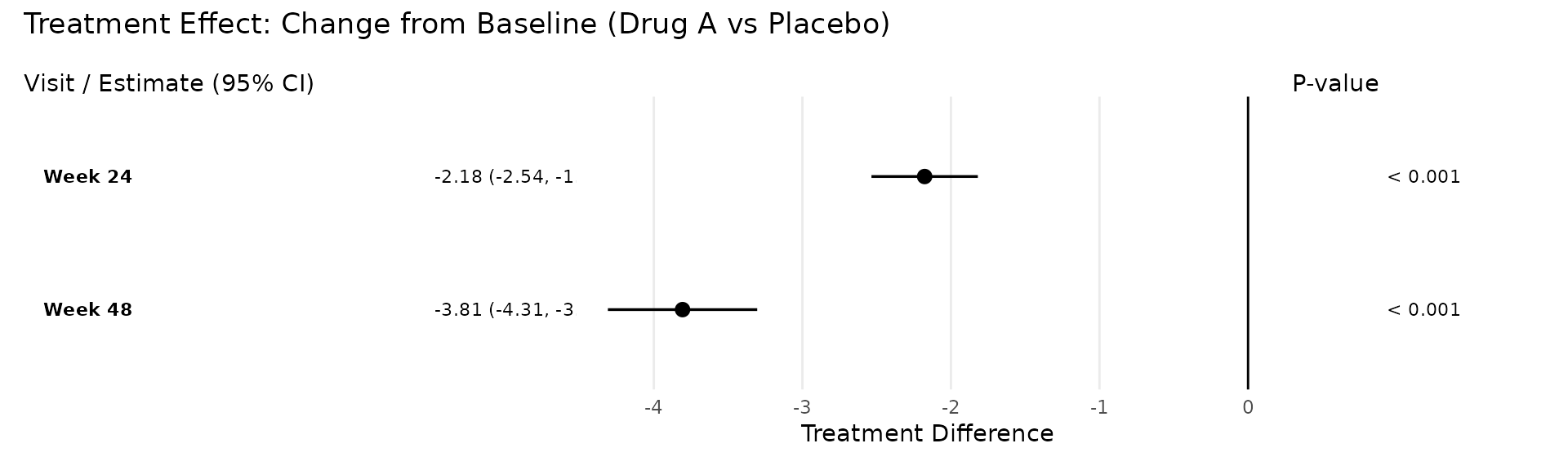
LS Mean Display Mode
The display = "lsm" mode shows the LS mean estimates for
each treatment arm, colour-coded using the Okabe-Ito
colourblind-friendly palette.
p_lsm <- plot_forest(
  pool_obj,
  display = "lsm",
  arm_labels = c(ref = "Placebo", alt = "Drug A"),
  title = "LS Mean Estimates by Visit"
)
p_lsm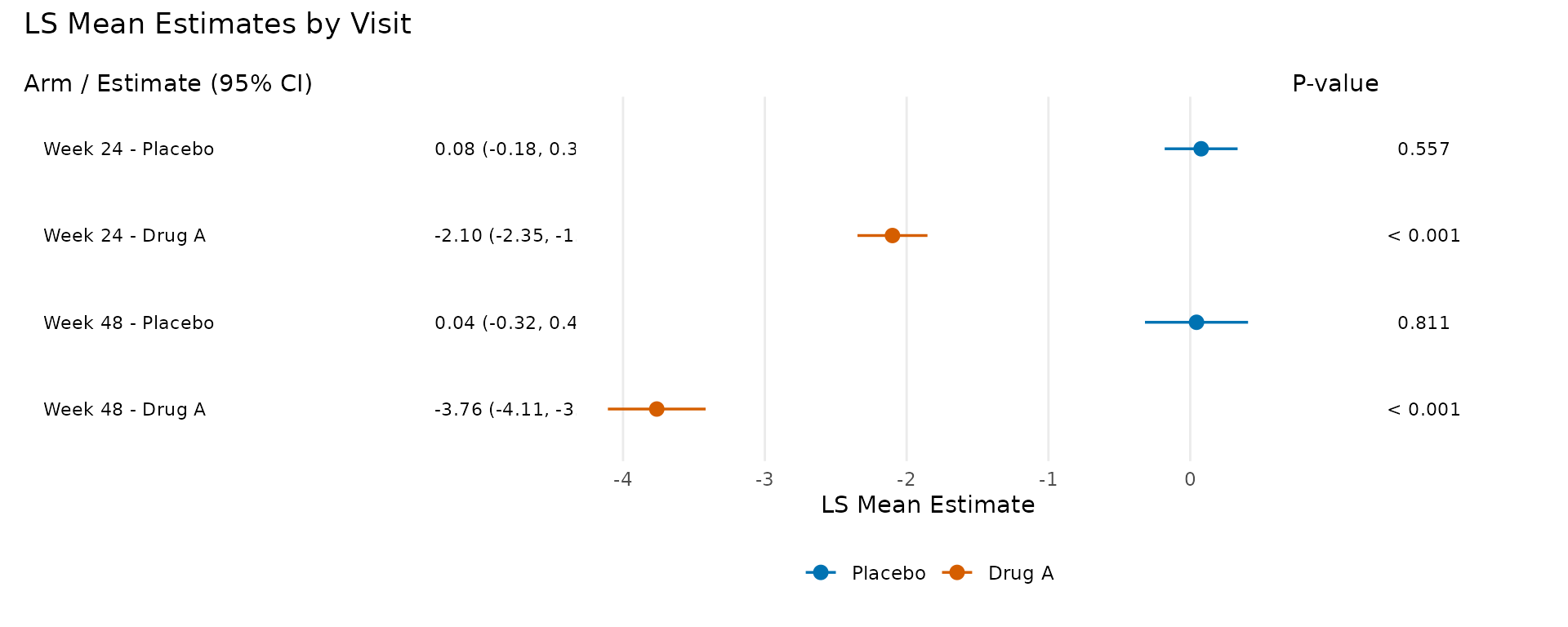
Both plot modes return a patchwork object that you can further
customise using the & theme() operator. For example, to
increase the text size across all panels:
plot_forest(pool_obj) & ggplot2::theme(text = ggplot2::element_text(size = 14))Binary/Responder Analysis
For binary responder endpoints using g-computation, see the deriving endpoints vignette, which
demonstrates how to define responder thresholds and analyse them using
the same reporting functions (efficacy_table(),
plot_forest()).