Comparison of Bayesian and frequentist MMRM fits
08/02/2024
Source:vignettes/comparison.Rmd
comparison.RmdAbout
This vignette provides an example comparison of a Bayesian MMRM fit,
obtained by brms.mmrm::brm_model(), and a frequentist MMRM
fit, obtained by mmrm::mmrm(). An overview of parameter
estimates and differences by type of MMRM is given in the summary (Table 4) at the end.
Prerequisites
Load required packages:
> packages <- c(
+   "dplyr",
+   "tidyr",
+   "ggplot2",
+   "gt",
+   "gtsummary",
+   "purrr",
+   "parallel",
+   "brms.mmrm",
+   "mmrm",
+   "emmeans",
+   "posterior"
+ )
> invisible(lapply(packages, library, character.only = TRUE))
Set seed:
> set.seed(123L)Data
Pre-processing
The fev_dat dataset is used that is contained in the
mmrm-package:
> data(fev_data, package = "mmrm")It is an artificial (simulated) dataset of a clinical trial
investigating the effect of an active treatment on FEV1
(forced expired volume in one second), compared to placebo.
FEV1 is a measure of how quickly the lungs can be emptied
and low levels may indicate chronic obstructive pulmonary disease
(COPD).
The dataset is a tibble with 800 rows and 7
variables:
-
USUBJID(subject ID), -
AVISIT(visit number), -
ARMCD(treatment,TRTorPBO), -
RACE(3-category race), -
SEX(sex), -
FEV1_BL(FEV1 at baseline, %), -
FEV1(FEV1 at study visits), -
WEIGHT(weighting variable).
In this analysis, change from baseline in FEV1 is used
as an endpoint and a corresponding new variable (FEV1_CHG)
is created.
Create and preprocess dataset for MMRM analysis:
> fev_data <- fev_data |>
+   mutate("FEV1_CHG" = FEV1 - FEV1_BL)
> fev_data <- brm_data(
+   data = fev_data,
+   outcome = "FEV1_CHG",
+   role = "change",
+   group = "ARMCD",
+   time = "AVISIT",
+   patient = "USUBJID",
+   baseline = "FEV1_BL",
+   reference_group = "PBO",
+   covariates = c("RACE", "SEX")
+ ) |>
+   mutate(ARMCD = factor(ARMCD), AVISIT = factor(AVISIT))
First rows of dataset:
> head(fev_data) |>
+   gt() |>
+ tab_caption(caption = md("Table 1. First rows of dataset."))| FEV1_CHG | FEV1_BL | ARMCD | AVISIT | USUBJID | RACE | SEX |
|---|---|---|---|---|---|---|
| NA | 45.02477 | PBO | VIS1 | PT2 | Asian | Male |
| -13.569552 | 45.02477 | PBO | VIS2 | PT2 | Asian | Male |
| -8.145878 | 45.02477 | PBO | VIS3 | PT2 | Asian | Male |
| 3.783324 | 45.02477 | PBO | VIS4 | PT2 | Asian | Male |
| NA | 43.50070 | PBO | VIS1 | PT3 | Black or African American | Female |
| -7.513705 | 43.50070 | PBO | VIS2 | PT3 | Black or African American | Female |
Descriptive statistics
Table of baseline characteristics:
> fev_data |>
+   select(ARMCD, USUBJID, SEX, RACE, FEV1_BL) |>
+   distinct() |>
+   select(-USUBJID) |>
+   tbl_summary(
+     by = c(ARMCD),
+     statistic = list(
+       all_continuous() ~ "{mean} ({sd})",
+       all_categorical() ~ "{n} / {N} ({p}%)"
+     )
+   ) |>
+ modify_caption("Table 2. Baseline characteristics.")| Characteristic | PBO, N = 1051 | TRT, N = 951 |
|---|---|---|
| SEX | ||
| Male | 50 / 105 (48%) | 44 / 95 (46%) |
| Female | 55 / 105 (52%) | 51 / 95 (54%) |
| RACE | ||
| Asian | 38 / 105 (36%) | 32 / 95 (34%) |
| Black or African American | 46 / 105 (44%) | 29 / 95 (31%) |
| White | 21 / 105 (20%) | 34 / 95 (36%) |
| FEV1_BL | 40 (9) | 40 (9) |
| 1 n / N (%); Mean (SD) | ||
Table of change from baseline in FEV1 over 52 weeks:
> fev_data |>
+   pull(AVISIT) |>
+   unique() |>
+   sort() |>
+   purrr::map(
+     .f = ~ fev_data |>
+       filter(AVISIT %in% .x) |>
+       tbl_summary(
+         by = ARMCD,
+         include = FEV1_CHG,
+         type = FEV1_CHG ~ "continuous2",
+         statistic = FEV1_CHG ~ c("{mean} ({sd})",
+                                  "{median} ({p25}, {p75})",
+                                  "{min}, {max}"),
+         label = list(FEV1_CHG = paste("Visit ", .x))
+       )
+   ) |>
+   tbl_stack(quiet = TRUE) |>
+ modify_caption("Table 3. Change from baseline.")| Characteristic | PBO, N = 105 | TRT, N = 95 |
|---|---|---|
| Visit VIS1 | ||
| Mean (SD) | -8 (9) | -2 (10) |
| Median (IQR) | -9 (-16, 0) | -4 (-9, 7) |
| Range | -26, 12 | -24, 20 |
| Unknown | 37 | 29 |
| Visit VIS2 | ||
| Mean (SD) | -3 (8) | 2 (9) |
| Median (IQR) | -3 (-10, 1) | 2 (-3, 8) |
| Range | -20, 15 | -22, 23 |
| Unknown | 36 | 24 |
| Visit VIS3 | ||
| Mean (SD) | 2 (8) | 5 (9) |
| Median (IQR) | 2 (-2, 8) | 6 (0, 11) |
| Range | -15, 20 | -19, 30 |
| Unknown | 34 | 37 |
| Visit VIS4 | ||
| Mean (SD) | 8 (12) | 13 (13) |
| Median (IQR) | 6 (1, 18) | 12 (5, 22) |
| Range | -20, 39 | -14, 47 |
| Unknown | 38 | 28 |
> fev_data |>
+   group_by(ARMCD) |>
+   ggplot(aes(x = AVISIT, y = FEV1_CHG, fill = factor(ARMCD))) +
+   geom_hline(yintercept = 0, col = "grey", size = 1.2) +
+   geom_boxplot(na.rm = TRUE) +
+   labs(x = "Visit",
+        y = "Change from baseline in FEV1",
+        fill = "Treatment") +
+   scale_fill_manual(values = c("darkgoldenrod2", "coral2")) +
+   theme_bw()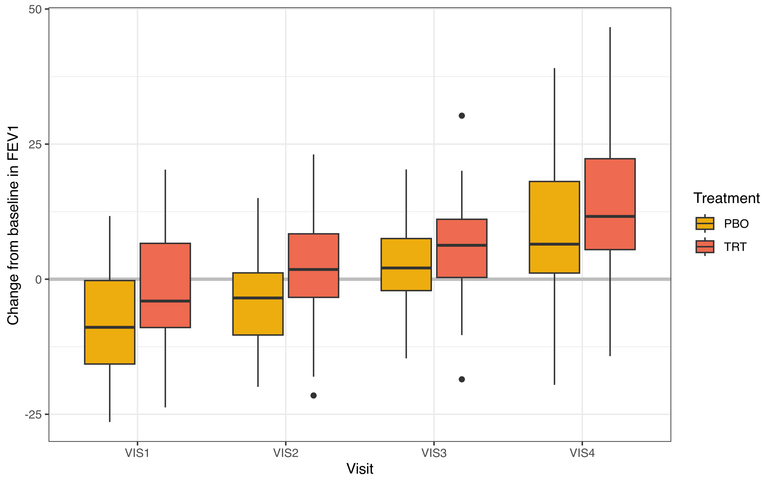
Figure 1. Change from baseline in FEV1 over 4 visit time points.
Fitting MMRMs
Bayesian model
Model formula:
> b_mmrm_formula <- brm_formula(
+   data = fev_data,
+   intercept = TRUE,
+   baseline = TRUE,
+   group = FALSE,
+   time = TRUE,
+   baseline_time = FALSE,
+   group_time = TRUE,
+   correlation = "unstructured"
+ )
> print(b_mmrm_formula)
FEV1_CHG ~ FEV1_BL + ARMCD:AVISIT + AVISIT + RACE + SEX + unstr(time = AVISIT, gr = USUBJID)
sigma ~ 0 + AVISIT
Fit model (using multiple cores, if available, to avoid long runtime):
> n_cores <- ifelse(
+   test = detectCores() > 1,
+   yes = min(2, detectCores()),
+   no = 1
+ )
> b_mmrm_fit <- brm_model(
+ data = filter(fev_data, !is.na(FEV1_CHG)),
+ formula = b_mmrm_formula,
+ iter = 1500,
+ chains = max(1, n_cores),
+ cores = n_cores,
+ refresh = 0
+ )Summary of results:
> summary(b_mmrm_fit)
 Family: gaussian
  Links: mu = identity; sigma = log
Formula: FEV1_CHG ~ FEV1_BL + ARMCD:AVISIT + AVISIT + RACE + SEX + unstr(time = AVISIT, gr = USUBJID)
         sigma ~ 0 + AVISIT
   Data: data[!is.na(data[[attr(data, "brm_outcome")]]), ] (Number of observations: 537)
  Draws: 2 chains, each with iter = 1500; warmup = 750; thin = 1;
         total post-warmup draws = 1500

Correlation Structures:
                   Estimate Est.Error l-95% CI u-95% CI Rhat Bulk_ESS Tail_ESS
cortime(VIS1,VIS2)     0.36      0.08     0.19     0.52 1.00     2550     1229
cortime(VIS1,VIS3)     0.14      0.10    -0.06     0.31 1.00     3032     1305
cortime(VIS2,VIS3)     0.04      0.10    -0.16     0.23 1.00     1928     1012
cortime(VIS1,VIS4)     0.17      0.11    -0.06     0.39 1.00     2638     1262
cortime(VIS2,VIS4)     0.11      0.09    -0.06     0.28 1.00     2404     1204
cortime(VIS3,VIS4)     0.01      0.10    -0.17     0.21 1.01     2579      855

Population-Level Effects:
                           Estimate Est.Error l-95% CI u-95% CI Rhat Bulk_ESS Tail_ESS
Intercept                     24.36      1.49    21.47    27.06 1.00     2163     1045
FEV1_BL                       -0.84      0.03    -0.90    -0.78 1.00     2979     1213
AVISITVIS2                     4.80      0.86     3.13     6.49 1.00     1604     1119
AVISITVIS3                    10.37      0.88     8.61    12.12 1.00     1338      877
AVISITVIS4                    15.16      1.30    12.62    17.79 1.00     1755     1273
RACEBlackorAfricanAmerican     1.40      0.58     0.29     2.54 1.00     1983     1032
RACEWhite                      5.44      0.61     4.31     6.64 1.00     2341     1238
SEXFemale                      0.35      0.51    -0.63     1.36 1.00     2932      965
AVISITVIS1:ARMCDTRT            3.98      1.10     1.78     6.10 1.00     1586      960
AVISITVIS2:ARMCDTRT            3.93      0.86     2.22     5.53 1.00     2091      838
AVISITVIS3:ARMCDTRT            2.98      0.67     1.66     4.33 1.00     3024     1304
AVISITVIS4:ARMCDTRT            4.46      1.66     1.22     7.72 1.01     2110     1307
sigma_AVISITVIS1               1.83      0.06     1.72     1.96 1.00     2312     1088
sigma_AVISITVIS2               1.59      0.06     1.48     1.71 1.00     2553     1228
sigma_AVISITVIS3               1.33      0.06     1.20     1.45 1.00     2458     1188
sigma_AVISITVIS4               2.28      0.06     2.17     2.40 1.00     2565     1006

Draws were sampled using sampling(NUTS). For each parameter, Bulk_ESS
and Tail_ESS are effective sample size measures, and Rhat is the potential
scale reduction factor on split chains (at convergence, Rhat = 1).
Frequentist model
Fit model:
> f_mmrm_fit <- mmrm::mmrm(
+   formula = FEV1_CHG ~ FEV1_BL + AVISIT + ARMCD:AVISIT + RACE + SEX +
+     us(AVISIT | USUBJID),
+   data = fev_data
+ )
Summary of results:
> summary(f_mmrm_fit)
mmrm fit

Formula:     FEV1_CHG ~ FEV1_BL + AVISIT + ARMCD:AVISIT + RACE + SEX + us(AVISIT |      USUBJID)
Data:        fev_data (used 537 observations from 197 subjects with maximum 4 timepoints)
Covariance:  unstructured (10 variance parameters)
Method:      Satterthwaite
Vcov Method: Asymptotic
Inference:   REML

Model selection criteria:
     AIC      BIC   logLik deviance
  3381.4   3414.2  -1680.7   3361.4

Coefficients:
                               Estimate Std. Error        df t value Pr(>|t|)
(Intercept)                    24.35372    1.40754 257.97000  17.302  < 2e-16 ***
FEV1_BL                        -0.84022    0.02777 190.27000 -30.251  < 2e-16 ***
AVISITVIS2                      4.79036    0.79848 144.82000   5.999 1.51e-08 ***
AVISITVIS3                     10.36601    0.81318 157.08000  12.748  < 2e-16 ***
AVISITVIS4                     15.19231    1.30857 139.25000  11.610  < 2e-16 ***
RACEBlack or African American   1.41921    0.57874 169.56000   2.452 0.015211 *
RACEWhite                       5.45679    0.61626 157.54000   8.855 1.65e-15 ***
SEXFemale                       0.33812    0.49273 166.43000   0.686 0.493529
AVISITVIS1:ARMCDTRT             3.98329    1.04540 142.32000   3.810 0.000206 ***
AVISITVIS2:ARMCDTRT             3.93076    0.81351 142.26000   4.832 3.46e-06 ***
AVISITVIS3:ARMCDTRT             2.98372    0.66567 129.61000   4.482 1.61e-05 ***
AVISITVIS4:ARMCDTRT             4.40400    1.66049 132.88000   2.652 0.008970 **
---
Signif. codes:  0 '***' 0.001 '**' 0.01 '*' 0.05 '.' 0.1 ' ' 1

Covariance estimate:
        VIS1    VIS2    VIS3    VIS4
VIS1 37.8301 11.3255  3.4796 10.6844
VIS2 11.3255 23.5476  0.7760  5.5103
VIS3  3.4796  0.7760 13.8037  0.5683
VIS4 10.6844  5.5103  0.5683 92.9625
Comparison
Extract estimates from Bayesian model
> b_mmrm_draws <- b_mmrm_fit |> as_draws_df()
> visit_levels <- sort(unique(as.character(fev_data$AVISIT)))
> for (level in visit_levels) {
+   name <- paste0("b_sigma_AVISIT", level)
+   b_mmrm_draws[[name]] <- exp(b_mmrm_draws[[name]])
+ }
> b_mmrm_summary <- b_mmrm_draws |>
+   summarize_draws() |>
+   select(variable, mean, sd) |>
+   filter(!(variable %in% c("lprior", "lp__"))) |>
+   rename(bayes_estimate = mean, bayes_se = sd) |>
+   mutate(
+     variable = variable |>
+       tolower() |>
+       gsub(pattern = "b_", replacement = "") |>
+       gsub(pattern = "b_sigma_AVISIT", replacement = "sigma_") |>
+       gsub(pattern = "cortime", replacement = "correlation") |>
+       gsub(pattern = "__", replacement = "_")
+   )
Extract estimates from frequentist model
> f_mmrm_fixed <- summary(f_mmrm_fit)$coefficients |>
+   as_tibble(rownames = "variable") |>
+   mutate(variable = tolower(variable)) |>
+   mutate(variable = gsub("(", "", variable, fixed = TRUE)) |>
+   mutate(variable = gsub(")", "", variable, fixed = TRUE)) |>
+   rename(freq_estimate = Estimate, freq_se = `Std. Error`) |>
+   select(variable, freq_estimate, freq_se)
> f_mmrm_variance <- tibble(
+ variable = paste0("sigma_AVISIT", visit_levels) |> tolower(),
+ freq_estimate = sqrt(diag(f_mmrm_fit$cov))
+ )> f_diagonal_factor <- diag(1 / sqrt(diag(f_mmrm_fit$cov)))
> f_corr_matrix <- f_diagonal_factor %*% f_mmrm_fit$cov %*% f_diagonal_factor
> colnames(f_corr_matrix) <- visit_levels> f_mmrm_correlation <- f_corr_matrix |>
+ as.data.frame() |>
+ as_tibble() |>
+ mutate(x1 = visit_levels) |>
+ pivot_longer(cols = -any_of("x1"),
+ names_to = "x2",
+ values_to = "freq_estimate") |>
+ filter(as.numeric(gsub("[^0-9]", "", x1)) <
+ as.numeric(gsub("[^0-9]", "", x2))) |>
+ mutate(variable = sprintf("correlation_%s_%s", x1, x2)) |>
+ select(variable, freq_estimate)> f_mmrm_summary <- bind_rows(f_mmrm_fixed,
+ f_mmrm_variance,
+ f_mmrm_correlation) |>
+ mutate(variable = gsub("\\s+", "", variable) |> tolower())Summary
> b_f_comparison <- full_join(x = b_mmrm_summary,
+                             y = f_mmrm_summary,
+                             by = "variable") |>
+   mutate(diff_estimate = bayes_estimate - freq_estimate,
+          diff_se = bayes_se - freq_se) |>
+   select(variable, ends_with("estimate"), ends_with("se"))
> gt(b_f_comparison) |>
+ fmt_number(decimals = 4) |>
+ tab_caption(
+ caption = md("Table 4. Contrasting Bayesian and frequentist MMRM fits.")
+ ) |>
+ tab_spanner(label = "Estimate", columns = ends_with("estimate")) |>
+ tab_spanner(label = "Standard error", columns = ends_with("se")) |>
+ cols_label(
+ variable = "Variable",
+ bayes_estimate = "Bayesian",
+ freq_estimate = "Frequentist",
+ diff_estimate = "Difference",
+ bayes_se = "Bayesian",
+ freq_se = "Frequentist",
+ diff_se = "Difference",
+ )| Variable | Estimate | Standard error | ||||
|---|---|---|---|---|---|---|
| Bayesian | Frequentist | Difference | Bayesian | Frequentist | Difference | |
| intercept | 24.3603 | 24.3537 | 0.0066 | 1.4858 | 1.4075 | 0.0783 |
| fev1_bl | −0.8403 | −0.8402 | −0.0001 | 0.0300 | 0.0278 | 0.0023 |
| avisitvis2 | 4.7974 | 4.7904 | 0.0071 | 0.8592 | 0.7985 | 0.0608 |
| avisitvis3 | 10.3694 | 10.3660 | 0.0034 | 0.8766 | 0.8132 | 0.0634 |
| avisitvis4 | 15.1647 | 15.1923 | −0.0276 | 1.2965 | 1.3086 | −0.0121 |
| raceblackorafricanamerican | 1.4031 | 1.4192 | −0.0161 | 0.5791 | 0.5787 | 0.0004 |
| racewhite | 5.4414 | 5.4568 | −0.0153 | 0.6116 | 0.6163 | −0.0047 |
| sexfemale | 0.3467 | 0.3381 | 0.0086 | 0.5137 | 0.4927 | 0.0210 |
| avisitvis1:armcdtrt | 3.9849 | 3.9833 | 0.0016 | 1.0980 | 1.0454 | 0.0526 |
| avisitvis2:armcdtrt | 3.9304 | 3.9308 | −0.0004 | 0.8612 | 0.8135 | 0.0477 |
| avisitvis3:armcdtrt | 2.9806 | 2.9837 | −0.0031 | 0.6722 | 0.6657 | 0.0065 |
| avisitvis4:armcdtrt | 4.4569 | 4.4040 | 0.0529 | 1.6552 | 1.6605 | −0.0053 |
| sigma_avisitvis1 | 6.2406 | 6.1506 | 0.0900 | 0.3997 | NA | NA |
| sigma_avisitvis2 | 4.9176 | 4.8526 | 0.0650 | 0.3011 | NA | NA |
| sigma_avisitvis3 | 3.7739 | 3.7153 | 0.0586 | 0.2386 | NA | NA |
| sigma_avisitvis4 | 9.7840 | 9.6417 | 0.1423 | 0.5906 | NA | NA |
| correlation_vis1_vis2 | 0.3617 | 0.3795 | −0.0177 | 0.0843 | NA | NA |
| correlation_vis1_vis3 | 0.1385 | 0.1523 | −0.0138 | 0.0956 | NA | NA |
| correlation_vis2_vis3 | 0.0400 | 0.0430 | −0.0031 | 0.0980 | NA | NA |
| correlation_vis1_vis4 | 0.1728 | 0.1802 | −0.0074 | 0.1138 | NA | NA |
| correlation_vis2_vis4 | 0.1123 | 0.1178 | −0.0054 | 0.0878 | NA | NA |
| correlation_vis3_vis4 | 0.0132 | 0.0159 | −0.0026 | 0.0977 | NA | NA |