A mixed model of repeated measures (MMRM) analyzes longitudinal clinical trial data. In a longitudinal dataset, there are multiple patients, and each patient has multiple observations at a common set of discrete points in time.
Raw data
To use the brms.mmrm package, begin with a longitudinal
dataset with one row per patient observation and columns for the
response variable, treatment group indicator, discrete time point
indicator, patient ID variable, and optional baseline covariates such as
age and gender. As an example, consider the fev_dat dataset
from the mmrm package.
data(fev_data, package = "mmrm")It is an artificial (simulated) dataset of a clinical trial
investigating the effect of an active treatment on FEV1
(forced expired volume in one second), compared to placebo.
FEV1 is a measure of how quickly the lungs can be emptied
and low levels may indicate chronic obstructive pulmonary disease
(COPD).
The dataset is a tibble with 800 rows and the following
notable variables:
-
USUBJID(subject ID) -
AVISIT(visit number, factor) -
VISITN(visit number, numeric) -
ARMCD(treatment,TRTorPBO) -
RACE(3-category race) -
SEX(female or male) -
FEV1_BL(FEV1 at baseline, %) -
FEV1(FEV1 at study visits) -
WEIGHT(weighting variable)
For this vignette, we derive the response variable
FEV1_CHG as the change from baseline of
FEV1.
fev_data <- fev_data |>
  mutate(FEV1_CHG = FEV1 - FEV1_BL)
Preprocessing
We use the brm_data() function to preprocess the raw
data and express it in a special classed data frame for
brms.mmrm. brm_data() stores arguments
outcome, group, time, etc. as
attributes which the downstream post-processing functions will
recognize.
data <- brm_data(
  data = fev_data,
  outcome = "FEV1_CHG",
  group = "ARMCD",
  time = "AVISIT",
  patient = "USUBJID",
  baseline = "FEV1_BL",
  reference_group = "PBO",
  reference_time = "VIS1",
  covariates = c("RACE", "SEX")
)
data
#> # A tibble: 800 × 11
#>    USUBJID AVISIT ARMCD RACE            SEX   FEV1_BL  FEV1 WEIGHT VISITN VISITN2 FEV1_CHG
#>    <fct>   <fct>  <fct> <fct>           <fct>   <dbl> <dbl>  <dbl>  <int>   <dbl>    <dbl>
#>  1 PT2     VIS1   PBO   Asian           Male     45.0  NA    0.465      1  0.330     NA
#>  2 PT2     VIS2   PBO   Asian           Male     45.0  31.5  0.233      2 -0.820    -13.6
#>  3 PT2     VIS3   PBO   Asian           Male     45.0  36.9  0.360      3  0.487     -8.15
#>  4 PT2     VIS4   PBO   Asian           Male     45.0  48.8  0.507      4  0.738      3.78
#>  5 PT3     VIS1   PBO   Black or Afric… Fema…    43.5  NA    0.682      1  0.576     NA
#>  6 PT3     VIS2   PBO   Black or Afric… Fema…    43.5  36.0  0.892      2 -0.305     -7.51
#>  7 PT3     VIS3   PBO   Black or Afric… Fema…    43.5  NA    0.128      3  1.51      NA
#>  8 PT3     VIS4   PBO   Black or Afric… Fema…    43.5  37.2  0.222      4  0.390     -6.34
#>  9 PT5     VIS1   PBO   Black or Afric… Male     43.6  32.3  0.411      1 -0.0162   -11.3
#> 10 PT5     VIS2   PBO   Black or Afric… Male     43.6  NA    0.422      2  0.944     NA
#> # ℹ 790 more rows
str(attributes(data))
#> List of 11
#>  $ row.names          : int [1:800] 1 2 3 4 5 6 7 8 9 10 ...
#>  $ names              : chr [1:11] "USUBJID" "AVISIT" "ARMCD" "RACE" ...
#>  $ class              : chr [1:4] "brms_mmrm_data" "tbl_df" "tbl" "data.frame"
#>  $ brm_outcome        : chr "FEV1_CHG"
#>  $ brm_baseline       : chr "FEV1_BL"
#>  $ brm_group          : chr "ARMCD"
#>  $ brm_time           : chr "AVISIT"
#>  $ brm_patient        : chr "USUBJID"
#>  $ brm_covariates     : chr [1:2] "RACE" "SEX"
#>  $ brm_reference_group: chr "PBO"
#>  $ brm_reference_time : chr "VIS1"
In addition, we convert the discrete time variable
AVISIT to an ordered factor whose levels respect the
chronological order given by the continuous time variable
VISITN.
data <- data |>
  brm_data_chronologize(order = "VISITN")
AVISIT has a special contrasts attribute
generated by contr.treatment() to prevent base R from
automatically assigning the default but inappropriate
contr.poly() polynomial contrasts.
str(data$AVISIT)
#>  Ord.factor w/ 4 levels "VIS1"<"VIS2"<..: 1 2 3 4 1 2 3 4 1 2 ...
#>  - attr(*, "contrasts")= num [1:4, 1:3] 0 1 0 0 0 0 1 0 0 0 ...
#>   ..- attr(*, "dimnames")=List of 2
#>   .. ..$ : chr [1:4] "VIS1" "VIS2" "VIS3" "VIS4"
#>   .. ..$ : chr [1:3] "2" "3" "4"
Formula
Next, choose a brms model formula for the fixed effect
and variance parameters. The brm_formula() function from
brms.mmrm makes this process easier. For example, here is a
formula that omits baseline response and interaction terms.
brm_formula(
  data = data,
  baseline = FALSE,
  baseline_time = FALSE,
  group_time = FALSE
)
#> FEV1_CHG ~ ARMCD + AVISIT + RACE + SEX + unstr(time = AVISIT, gr = USUBJID)
#> sigma ~ 0 + AVISIT
For the purposes of our example, we choose a fully parameterized analysis of the raw response.
formula <- brm_formula(data = data)

formula
#> FEV1_CHG ~ FEV1_BL + FEV1_BL:AVISIT + ARMCD + ARMCD:AVISIT + AVISIT + RACE + SEX + unstr(time = AVISIT, gr = USUBJID)
#> sigma ~ 0 + AVISIT
Priors
Some analyses require informative priors, others require
non-informative ones. Please use brms to construct
a prior suitable for your analysis. The brms package has
documentation on how its default priors are constructed and how to set
your own priors.1 Once you have an R object that represents
the joint prior distribution of your model, you can pass it to the
brm_model() function described below. The
get_prior() function shows the default priors for a given
dataset and model formula.
brms::get_prior(data = data, formula = formula) |>
  as.data.frame() |>
  select(-any_of(c("group", "resp", "nlpar", "lb", "ub", "source")))
#>                      prior     class                       coef  dpar
#> 1                                  b
#> 2                                  b                   ARMCDTRT
#> 3                                  b           ARMCDTRT:AVISIT2
#> 4                                  b           ARMCDTRT:AVISIT3
#> 5                                  b           ARMCDTRT:AVISIT4
#> 6                                  b                    AVISIT2
#> 7                                  b                    AVISIT3
#> 8                                  b                    AVISIT4
#> 9                                  b                    FEV1_BL
#> 10                                 b            FEV1_BL:AVISIT2
#> 11                                 b            FEV1_BL:AVISIT3
#> 12                                 b            FEV1_BL:AVISIT4
#> 13                                 b RACEBlackorAfricanAmerican
#> 14                                 b                  RACEWhite
#> 15                                 b                  SEXFemale
#> 16                  lkj(1)   cortime
#> 17 student_t(3, 1.9, 11.8) Intercept
#> 18                                 b                            sigma
#> 19                                 b                 AVISITVIS1 sigma
#> 20                                 b                 AVISITVIS2 sigma
#> 21                                 b                 AVISITVIS3 sigma
#> 22                                 b                 AVISITVIS4 sigma
Model
To run an MMRM, use the brm_model() function. This
function calls brms::brm() behind the scenes, using the
formula and prior you set in the formula and
prior arguments.
model <- brm_model(data = data, formula = formula, refresh = 0)
#> Compiling Stan program...
#> Start sampling
The result is a brms model object with extra list
elements brms.mmrm_data and brms.mmrm_formula
to keep track of the data and formula used to fit the model.
model
#>  Family: gaussian
#>   Links: mu = identity; sigma = log
#> Formula: FEV1_CHG ~ FEV1_BL + FEV1_BL:AVISIT + ARMCD + ARMCD:AVISIT + AVISIT + RACE + SEX + unstr(time = AVISIT, gr = USUBJID)
#>          sigma ~ 0 + AVISIT
#>    Data: modeled_data (Number of observations: 537)
#>   Draws: 4 chains, each with iter = 2000; warmup = 1000; thin = 1;
#>          total post-warmup draws = 4000
#>
#> Correlation Structures:
#>                    Estimate Est.Error l-95% CI u-95% CI Rhat Bulk_ESS Tail_ESS
#> cortime(VIS1,VIS2)     0.36      0.08     0.19     0.51 1.00     5330     3117
#> cortime(VIS1,VIS3)     0.14      0.10    -0.06     0.32 1.00     5545     2626
#> cortime(VIS2,VIS3)     0.04      0.10    -0.15     0.24 1.00     5103     3078
#> cortime(VIS1,VIS4)     0.16      0.12    -0.08     0.38 1.00     5353     2866
#> cortime(VIS2,VIS4)     0.11      0.09    -0.06     0.28 1.00     6012     3087
#> cortime(VIS3,VIS4)     0.01      0.10    -0.19     0.21 1.00     4506     2771
#>
#> Regression Coefficients:
#>                            Estimate Est.Error l-95% CI u-95% CI Rhat Bulk_ESS Tail_ESS
#> Intercept                     23.32      2.57    18.30    28.46 1.00     1595     2142
#> FEV1_BL                       -0.82      0.06    -0.93    -0.70 1.00     1720     2210
#> ARMCDTRT                       4.04      1.07     1.97     6.20 1.00     2694     3113
#> AVISIT2                        4.43      2.75    -1.15     9.82 1.00     2037     2470
#> AVISIT3                       12.55      2.93     6.74    18.27 1.00     1852     2195
#> AVISIT4                       15.59      4.23     7.38    23.91 1.00     2489     2521
#> RACEBlackorAfricanAmerican     1.45      0.59     0.28     2.65 1.00     5262     3112
#> RACEWhite                      5.46      0.61     4.26     6.68 1.00     5172     3218
#> SEXFemale                      0.38      0.51    -0.62     1.40 1.00     5881     3056
#> FEV1_BL:AVISIT2                0.01      0.06    -0.12     0.14 1.00     2069     2704
#> FEV1_BL:AVISIT3               -0.05      0.07    -0.19     0.08 1.00     1898     2215
#> FEV1_BL:AVISIT4               -0.01      0.10    -0.21     0.19 1.00     2596     2762
#> ARMCDTRT:AVISIT2              -0.06      1.15    -2.31     2.17 1.00     2894     3132
#> ARMCDTRT:AVISIT3              -1.02      1.20    -3.37     1.38 1.00     3078     3105
#> ARMCDTRT:AVISIT4               0.35      1.88    -3.30     3.93 1.00     3810     3176
#> sigma_AVISITVIS1               1.83      0.06     1.71     1.95 1.00     5127     3300
#> sigma_AVISITVIS2               1.59      0.06     1.47     1.71 1.00     5574     3239
#> sigma_AVISITVIS3               1.33      0.06     1.21     1.45 1.00     5217     3072
#> sigma_AVISITVIS4               2.28      0.06     2.16     2.41 1.00     6592     3198
#>
#> Draws were sampled using sampling(NUTS). For each parameter, Bulk_ESS
#> and Tail_ESS are effective sample size measures, and Rhat is the potential
#> scale reduction factor on split chains (at convergence, Rhat = 1).
model$brms.mmrm_data
#> # A tibble: 800 × 11
#>    USUBJID AVISIT ARMCD RACE            SEX   FEV1_BL  FEV1 WEIGHT VISITN VISITN2 FEV1_CHG
#>    <fct>   <ord>  <fct> <fct>           <fct>   <dbl> <dbl>  <dbl>  <int>   <dbl>    <dbl>
#>  1 PT2     VIS1   PBO   Asian           Male     45.0  NA    0.465      1  0.330     NA
#>  2 PT2     VIS2   PBO   Asian           Male     45.0  31.5  0.233      2 -0.820    -13.6
#>  3 PT2     VIS3   PBO   Asian           Male     45.0  36.9  0.360      3  0.487     -8.15
#>  4 PT2     VIS4   PBO   Asian           Male     45.0  48.8  0.507      4  0.738      3.78
#>  5 PT3     VIS1   PBO   Black or Afric… Fema…    43.5  NA    0.682      1  0.576     NA
#>  6 PT3     VIS2   PBO   Black or Afric… Fema…    43.5  36.0  0.892      2 -0.305     -7.51
#>  7 PT3     VIS3   PBO   Black or Afric… Fema…    43.5  NA    0.128      3  1.51      NA
#>  8 PT3     VIS4   PBO   Black or Afric… Fema…    43.5  37.2  0.222      4  0.390     -6.34
#>  9 PT5     VIS1   PBO   Black or Afric… Male     43.6  32.3  0.411      1 -0.0162   -11.3
#> 10 PT5     VIS2   PBO   Black or Afric… Male     43.6  NA    0.422      2  0.944     NA
#> # ℹ 790 more rows
model$brms.mmrm_formula
#> FEV1_CHG ~ FEV1_BL + FEV1_BL:AVISIT + ARMCD + ARMCD:AVISIT + AVISIT + RACE + SEX + unstr(time = AVISIT, gr = USUBJID)
#> sigma ~ 0 + AVISIT
Marginals
Regardless of the choice of fixed effects formula,
brms.mmrm performs inference on the marginal distributions
at each treatment group and time point of the mean of the following
quantities:
- Response.
- Change from baseline. Only reported if you originally declared a
baseline time point with the
reference_timeargument ofbrm_data(). - Treatment difference. If you declared a baseline in (2), then treatment difference is calculated in terms of change from baseline. Otherwise, it is calculated in terms of raw response.
- Effect size: treatment difference divided by the residual standard deviation.
To derive posterior draws of these marginals, use the
brm_marginal_draws() function.
draws <- brm_marginal_draws(model = model)

names(draws)
#> [1] "response"         "difference_time"  "difference_group" "effect"
#> [5] "sigma"

draws$difference_group
#> # A draws_df: 1000 iterations, 4 chains, and 3 variables
#>    TRT|VIS2 TRT|VIS3 TRT|VIS4
#> 1     0.251    -2.24    1.149
#> 2    -0.662    -1.33   -0.804
#> 3    -0.129    -1.57    2.736
#> 4    -0.370    -2.00    1.231
#> 5    -0.964    -1.91   -1.026
#> 6    -0.939    -1.15    0.258
#> 7    -0.026    -1.15   -0.047
#> 8     0.052    -1.48    1.239
#> 9    -0.929    -0.81   -0.791
#> 10   -0.437    -1.16    2.233
#> # ... with 3990 more draws
#> # ... hidden reserved variables {'.chain', '.iteration', '.draw'}
If you need samples from these marginals averaged across time points,
e.g. an “overall effect size”, brm_marginal_draws_average()
can average the draws above across discrete time points (either all or a
user-defined subset).
draws_average <- brm_marginal_draws_average(draws = draws, data = data)

names(draws_average)
#> [1] "response"         "difference_time"  "difference_group" "effect"
#> [5] "sigma"

draws_average$difference_group
#> # A draws_df: 1000 iterations, 4 chains, and 1 variables
#>    TRT|average
#> 1       -0.281
#> 2       -0.932
#> 3        0.347
#> 4       -0.380
#> 5       -1.300
#> 6       -0.610
#> 7       -0.407
#> 8       -0.064
#> 9       -0.845
#> 10       0.212
#> # ... with 3990 more draws
#> # ... hidden reserved variables {'.chain', '.iteration', '.draw'}
The brm_marginal_summaries() function produces posterior
summaries of these marginals, and it includes the Monte Carlo standard
error (MCSE) of each estimate.
summaries <- brm_marginal_summaries(draws, level = 0.95)

summaries
#> # A tibble: 140 × 6
#>    marginal         statistic group time    value   mcse
#>    <chr>            <chr>     <chr> <chr>   <dbl>  <dbl>
#>  1 difference_group lower     TRT   VIS2  -2.31   0.0465
#>  2 difference_group lower     TRT   VIS3  -3.37   0.0668
#>  3 difference_group lower     TRT   VIS4  -3.30   0.0688
#>  4 difference_group mean      TRT   VIS2  -0.0638 0.0216
#>  5 difference_group mean      TRT   VIS3  -1.02   0.0219
#>  6 difference_group mean      TRT   VIS4   0.348  0.0311
#>  7 difference_group median    TRT   VIS2  -0.0714 0.0249
#>  8 difference_group median    TRT   VIS3  -1.02   0.0252
#>  9 difference_group median    TRT   VIS4   0.381  0.0320
#> 10 difference_group sd        TRT   VIS2   1.15   0.0161
#> # ℹ 130 more rows
The brm_marginal_probabilities() function shows
posterior probabilities of the form,
or
brm_marginal_probabilities(
  draws = draws,
  threshold = c(-0.1, 0.1),
  direction = c("greater", "less")
)
#> # A tibble: 6 × 5
#>   direction threshold group time  value
#>   <chr>         <dbl> <chr> <chr> <dbl>
#> 1 greater        -0.1 TRT   VIS2  0.511
#> 2 greater        -0.1 TRT   VIS3  0.220
#> 3 greater        -0.1 TRT   VIS4  0.594
#> 4 less            0.1 TRT   VIS2  0.56
#> 5 less            0.1 TRT   VIS3  0.827
#> 6 less            0.1 TRT   VIS4  0.443
Finally, brm_marignal_data() computes marginal means and
confidence intervals on the response variable in the data, along with
other summary statistics.
summaries_data <- brm_marginal_data(data = data, level = 0.95)

summaries_data
#> # A tibble: 56 × 4
#>    statistic group time   value
#>    <chr>     <fct> <ord>  <dbl>
#>  1 lower     PBO   VIS1  -5.86
#>  2 lower     PBO   VIS2  -1.44
#>  3 lower     PBO   VIS3   4.33
#>  4 lower     PBO   VIS4  11.1
#>  5 lower     TRT   VIS1   0.423
#>  6 lower     TRT   VIS2   3.96
#>  7 lower     TRT   VIS3   7.67
#>  8 lower     TRT   VIS4  16.0
#>  9 mean      PBO   VIS1  -8.09
#> 10 mean      PBO   VIS2  -3.38
#> # ℹ 46 more rows
Visualization
Comparing models and data
Suppose we fit a second model which omits baseline.
summaries_no_baseline <- data |>
brm_formula(baseline = FALSE, baseline_time = FALSE) |>
brm_model(data = data, refresh = 0) |>
brm_marginal_draws() |>
brm_marginal_summaries()
#> Compiling Stan program...
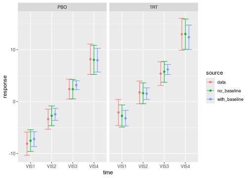
#> Start samplingThe brm_plot_compare() function compares means and
intervals from different models and data sources in the same plot.
brm_plot_compare(
  data = summaries_data,
  no_baseline = summaries_no_baseline,
  with_baseline = summaries
)
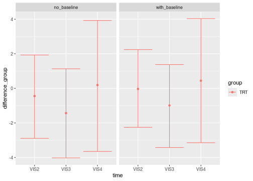
If you omit the marginals of the data, you can show inference on change from baseline or the treatment effect.
brm_plot_compare(
  no_baseline = summaries_no_baseline,
  with_baseline = summaries,
  marginal = "difference_group" # treatment effect
)
Additional arguments let you control the primary comparison of interest (the color aesthetic), the horizontal axis, and the faceting variable.
brm_plot_compare(
  no_baseline = summaries_no_baseline,
  with_baseline = summaries,
  marginal = "difference_group",
  compare = "group",
  axis = "time",
  facet = "source" # model1 vs model2
)
Plotting draws
brm_plot_draws() can plot the posterior draws of the
response, change from baseline, or treatment difference.
brm_plot_draws(draws = draws$difference_group)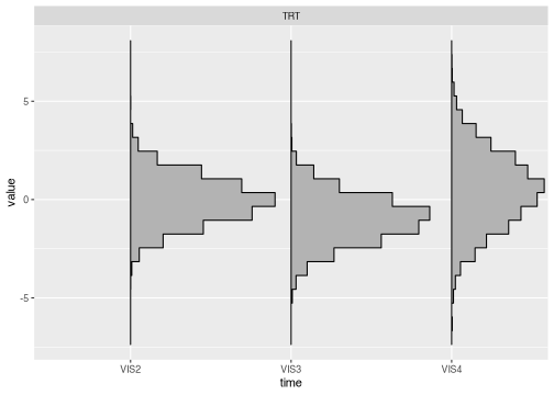
The axis and facet arguments customize the
horizontal axis and faceting variable, respectively.
brm_plot_draws(
  draws = draws$difference_group,
  axis = "group",
  facet = "time"
)
Comparing priors and posteriors
For a model with an intercept term and with automatic centering in
brms turned on, brms by default assigns a
mildly informative Student t prior to help the MCMC converge.2
brms::prior_summary(model) |>
  filter(class == "Intercept")
#> Intercept ~ student_t(3, 1.9, 11.8)
Suppose we want to compare the prior on Intercept to its
marginal posterior. To begin, we express the prior using the
distributional package, extract posterior samples from the
brms model, and visualize them together with the
ggdist package. Below, the shaded gray region is the
posterior density, and the blue line is the prior density.
library(distributional)
library(ggdist)
library(ggplot2)
library(posterior)

prior <- dist_student_t(3, 1.9, 11.8)
posterior <- as_draws_df(model)

ggplot() +
  stat_halfeye(aes(x = Intercept), data = posterior) +
  stat_slab(aes(xdist = prior), color = "blue", fill = NA) +
  scale_thickness_shared()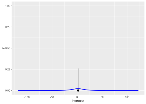
Appendix A: Contrasts
The formula is not the only factor that ultimately determines the
fixed effect parameterization. The ordering of the categorical variables
in the data, as well as the contrast option in R, affect
the construction of the model matrix. To see the model matrix that will
ultimately be used in brm_model(), run
brms::make_standata() and examine the X
element of the returned list.
The contrast option accepts a named vector of two
character vectors which govern model.matrix() contrasts for
unordered and ordered variables, respectively.
The make_standata() function lets you see the data that
brms will generate for Stan. This includes the fixed
effects model matrix X. Note the differences in the
groupgroup_* additive terms between the matrix below and
the one above.
head(brms::make_standata(formula = formula, data = data)$X)
#>     Intercept  FEV1_BL ARMCDPBO AVISIT2 AVISIT3 AVISIT4 RACEAsian
#> 422         1 25.27144        0       1       0       0         0
#> 424         1 25.27144        0       0       0       1         0
#> 2           1 45.02477        1       1       0       0         1
#> 3           1 45.02477        1       0       1       0         1
#> 4           1 45.02477        1       0       0       1         1
#> 6           1 43.50070        1       1       0       0         0
#>     RACEBlackorAfricanAmerican SEXMale FEV1_BL:AVISIT2 FEV1_BL:AVISIT3 FEV1_BL:AVISIT4
#> 422                          1       0        25.27144         0.00000         0.00000
#> 424                          1       0         0.00000         0.00000        25.27144
#> 2                            0       1        45.02477         0.00000         0.00000
#> 3                            0       1         0.00000        45.02477         0.00000
#> 4                            0       1         0.00000         0.00000        45.02477
#> 6                            1       0        43.50070         0.00000         0.00000
#>     ARMCDPBO:AVISIT2 ARMCDPBO:AVISIT3 ARMCDPBO:AVISIT4
#> 422                0                0                0
#> 424                0                0                0
#> 2                  1                0                0
#> 3                  0                1                0
#> 4                  0                0                1
#> 6                  1                0                0
If you choose a different contrast method, a different model matrix may result.
options(
  contrasts = c(unordered = "contr.treatment", ordered = "contr.poly")
)
# different model matrix than before:
head(brms::make_standata(formula = formula, data = data)$X)
#>     Intercept  FEV1_BL ARMCDTRT AVISIT2 AVISIT3 AVISIT4 RACEBlackorAfricanAmerican
#> 422         1 25.27144        1       1       0       0                          1
#> 424         1 25.27144        1       0       0       1                          1
#> 2           1 45.02477        0       1       0       0                          0
#> 3           1 45.02477        0       0       1       0                          0
#> 4           1 45.02477        0       0       0       1                          0
#> 6           1 43.50070        0       1       0       0                          1
#>     RACEWhite SEXFemale FEV1_BL:AVISIT2 FEV1_BL:AVISIT3 FEV1_BL:AVISIT4 ARMCDTRT:AVISIT2
#> 422         0         1        25.27144         0.00000         0.00000                1
#> 424         0         1         0.00000         0.00000        25.27144                0
#> 2           0         0        45.02477         0.00000         0.00000                0
#> 3           0         0         0.00000        45.02477         0.00000                0
#> 4           0         0         0.00000         0.00000        45.02477                0
#> 6           0         1        43.50070         0.00000         0.00000                0
#>     ARMCDTRT:AVISIT3 ARMCDTRT:AVISIT4
#> 422                0                0
#> 424                0                1
#> 2                  0                0
#> 3                  0                0
#> 4                  0                0
#> 6                  0                0
Recall from earlier that brm_data_chronologize()
protects the discrete time variable (in our case, AVISIT)
from the contrasts option by assigning a
contrasts attribute of its own.
str(data$AVISIT)
#>  Ord.factor w/ 4 levels "VIS1"<"VIS2"<..: 1 2 3 4 1 2 3 4 1 2 ...
#>  - attr(*, "contrasts")= num [1:4, 1:3] 0 1 0 0 0 0 1 0 0 0 ...
#>   ..- attr(*, "dimnames")=List of 2
#>   .. ..$ : chr [1:4] "VIS1" "VIS2" "VIS3" "VIS4"
#>   .. ..$ : chr [1:3] "2" "3" "4"
Appendix B: Imputation of missing outcomes
Under the missing at random (MAR) assumptions, MMRMs do not require
imputation (Holzhauer and Weber (2024)).
However, if the outcomes in your data are not missing at random, or if
you are targeting an alternative estimand, then you may need to impute
missing outcomes. brms.mmrm can leverage either of the two
alternative solutions described at https://paulbuerkner.com/brms/articles/brms_missings.html.
Imputation before model fitting
To impute missing outcomes before model fitting, first use create a
list of imputed datasets using the multiple imputation method of your
choice. The rbmi
package is uniquely suited to the multiple imputation of continuous
longitudinal clinical trial data.
variables <- rbmi::set_vars(
  outcome = "FEV1_CHG",
  visit = "AVISIT",
  subjid = "USUBJID",
  group = "ARMCD",
  covariates = c("RACE", "SEX")
)
imputation_draws <- rbmi::draws(
  data = data |>
    mutate(
      USUBJID = as.factor(USUBJID),
      AVISIT = as.factor(AVISIT)
    ),
  vars = variables,
  method = rbmi::method_condmean(type = "jackknife"),
  quiet = TRUE
)
imputation_run <- rbmi::impute(
  draws = imputation_draws,
  references = c(
    placebo = "PBO",
    treatment = "TRT"
  )
)
imputed_datasets <- rbmi::extract_imputed_dfs(imputation_run)
At this point, imputed_datasets is a list of data frames
with the response variable imputed with multiple imputation. Simply
supply this list to the imputed argument of
brm_model(). Internally, brm_model() calls
brms::brm_multiple(data = imputed, formula = formula)
instead of brms::brm(data = data, formula = formula) to fit
an MMRM to each of the individual imputed datasets in the
imputed object. The computation could take several hours
because it requires many fitted MMRM.
model <- brm_model(
  data = data, # Yes, please supply the original non-imputed dataset too.
  formula = formula,
  imputed = imputed_datasets,
  refresh = 0
)
Unless you set combine = FALSE in
brm_model(), brms automatically combines
posterior samples across imputed datasets. This means the downstream
post-processing workflow below is exactly the same as the non-imputation
case.
Imputation during model fitting
Alternatively, to conduct imputation during the fitting of that
model, set model_missing_outcomes to TRUE in
brm_formula(). This formula uses
response | mi() instead of just response on
the left-hand side to tell brms to model each missing
outcome as a model parameter. To use this type of imputation, simply
supply the returned formula object to the formula argument
of brm_model().
brm_formula(data, model_missing_outcomes = TRUE)
#> FEV1_CHG | mi() ~ FEV1_BL + FEV1_BL:AVISIT + ARMCD + ARMCD:AVISIT + AVISIT + RACE + SEX + unstr(time = AVISIT, gr = USUBJID)
#> sigma ~ 0 + AVISIT
Unlike imputation before model fitting, this approach requires only one fit of the model. However, that model will sample posterior draws for each missing outcome as if it were a model parameter, so the MCMC may run slower and produce a larger output object.