Subgroup analysis • brms.mmrm

This vignette explains how to incorporate a subgroup variable into an MMRM using the brms.mmrm package. Here, we assume the subgroup variable has already been selected in advance (perhaps pre-specified in a trial protocol) because interactions are anticipated or of particular interest. Especially if heterogeneous patient populations are studied, it is important to check that the estimated overall effect is broadly applicable to relevant subgroups (ICH (1998), EMA (2019)). It is worth noting, however, that subgroup variable selection is a thorough process that requires deep domain knowledge, careful adjustments for multiplicity, and potentially different modeling approaches, all of which belongs outside the scope of this vignette. Limitations of one-variable-at-a-time subgroup analyses to detect treatment effect heterogeneity have been described in the literature (Kent 2023). For literature on data-driven subgroup identification methods in clinical trials, we refer to Lipkovich et al. (2017) and Lipkovich et al. (2023).

Data

The subgroup variable must be categorical.

library(brms.mmrm)
library(dplyr)
library(magrittr)
set.seed(0L)
raw_data <- brm_simulate_outline(
  n_group = 3,
  n_subgroup = 2,
  n_patient = 50,
  n_time = 3,
  rate_dropout = 0,
  rate_lapse = 0
) |>
  mutate(response = rnorm(n = n()))

raw_data
#> # A tibble: 900 × 6
#>    patient     time   group   subgroup   missing response
#>    <chr>       <chr>  <chr>   <chr>      <lgl>      <dbl>
#>  1 patient_001 time_1 group_1 subgroup_1 FALSE    1.26   
#>  2 patient_001 time_2 group_1 subgroup_1 FALSE   -0.326  
#>  3 patient_001 time_3 group_1 subgroup_1 FALSE    1.33   
#>  4 patient_002 time_1 group_1 subgroup_1 FALSE    1.27   
#>  5 patient_002 time_2 group_1 subgroup_1 FALSE    0.415  
#>  6 patient_002 time_3 group_1 subgroup_1 FALSE   -1.54   
#>  7 patient_003 time_1 group_1 subgroup_1 FALSE   -0.929  
#>  8 patient_003 time_2 group_1 subgroup_1 FALSE   -0.295  
#>  9 patient_003 time_3 group_1 subgroup_1 FALSE   -0.00577
#> 10 patient_004 time_1 group_1 subgroup_1 FALSE    2.40   
#> # ℹ 890 more rows

Each categorical subgroup level should have adequate representation among all treatment groups at all discrete time points. Otherwise, some marginal means of interest may not be estimable.

count(raw_data, group, subgroup, time)
#> # A tibble: 18 × 4
#>    group   subgroup   time       n
#>    <chr>   <chr>      <chr>  <int>
#>  1 group_1 subgroup_1 time_1    50
#>  2 group_1 subgroup_1 time_2    50
#>  3 group_1 subgroup_1 time_3    50
#>  4 group_1 subgroup_2 time_1    50
#>  5 group_1 subgroup_2 time_2    50
#>  6 group_1 subgroup_2 time_3    50
#>  7 group_2 subgroup_1 time_1    50
#>  8 group_2 subgroup_1 time_2    50
#>  9 group_2 subgroup_1 time_3    50
#> 10 group_2 subgroup_2 time_1    50
#> 11 group_2 subgroup_2 time_2    50
#> 12 group_2 subgroup_2 time_3    50
#> 13 group_3 subgroup_1 time_1    50
#> 14 group_3 subgroup_1 time_2    50
#> 15 group_3 subgroup_1 time_3    50
#> 16 group_3 subgroup_2 time_1    50
#> 17 group_3 subgroup_2 time_2    50
#> 18 group_3 subgroup_2 time_3    50

When you create the special classed dataset for brms.mmrm using brm_data(), please supply the name of the subgroup variable and a reference subgroup level. Post-processing functions will use the reference subgroup level to compare pairs of subgroups: for example, the treatment effect of subgroup_2 minus the treatment effect of the reference subgroup level you choose.

data <- brm_data(
  data = raw_data,
  outcome = "response",
  baseline = NULL,
  group = "group",
  subgroup = "subgroup",
  time = "time",
  patient = "patient",
  reference_group = "group_1",
  reference_subgroup = "subgroup_1",
  reference_time = "time_1"
)

str(data)
#> brms_mm_ [900 × 6] (S3: brms_mmrm_data/tbl_df/tbl/data.frame)
#>  $ patient : chr [1:900] "patient_001" "patient_001" "patient_001" "patient_002" ...
#>  $ time    : chr [1:900] "time_1" "time_2" "time_3" "time_1" ...
#>  $ group   : chr [1:900] "group_1" "group_1" "group_1" "group_1" ...
#>  $ subgroup: chr [1:900] "subgroup_1" "subgroup_1" "subgroup_1" "subgroup_1" ...
#>  $ missing : logi [1:900] FALSE FALSE FALSE FALSE FALSE FALSE ...
#>  $ response: num [1:900] 1.263 -0.326 1.33 1.272 0.415 ...
#>  - attr(*, "brm_outcome")= chr "response"
#>  - attr(*, "brm_group")= chr "group"
#>  - attr(*, "brm_subgroup")= chr "subgroup"
#>  - attr(*, "brm_time")= chr "time"
#>  - attr(*, "brm_patient")= chr "patient"
#>  - attr(*, "brm_covariates")= chr(0) 
#>  - attr(*, "brm_reference_group")= chr "group_1"
#>  - attr(*, "brm_reference_subgroup")= chr "subgroup_1"
#>  - attr(*, "brm_reference_time")= chr "time_1"

Formula

For subgroup analysis, the formula should have terms that include the subgroup variable. All plausible interactions are optional via arguments of brm_formula(). For this specific example, we disable all interactions except group-subgroup interaction.

formula_subgroup <- brm_formula(
  data = data,
  group_subgroup_time = FALSE,
  subgroup_time = FALSE
)

formula_subgroup
#> response ~ group + group:subgroup + group:time + subgroup + time + unstr(time = time, gr = patient) 
#> sigma ~ 0 + time

To create an analogous non-subgroup reduced model, disable each of the terms that involve the subgroup. This will be useful later on for measuring the impact of the subgroup as a whole, without needing to restrict to a specific level of the subgroup.¹

formula_reduced <- brm_formula(
  data = data,
  group_subgroup = FALSE,
  group_subgroup_time = FALSE,
  subgroup = FALSE,
  subgroup_time = FALSE
)

formula_reduced
#> response ~ group + group:time + time + unstr(time = time, gr = patient) 
#> sigma ~ 0 + time

Models

To run the full subgroup and reduced non-subgroup models, use brm_model() as usual. Remember to supply the appropriate formula to each case.

model_subgroup <- brm_model(
  data = data,
  formula = formula_subgroup,
  refresh = 0
)
#> Compiling Stan program...
#> Start sampling

model_reduced <- brm_model(
  data = data,
  formula = formula_reduced,
  refresh = 0
)
#> Compiling Stan program...
#> Start sampling

Marginals

brm_marginal_draws() automatically produces subgroup-specific marginal means if brm_formula() declared subgroup-specific fixed effects.²

draws_subgroup <- brm_marginal_draws(
  model = model_subgroup,
  average_within_subgroup = FALSE
)

draws_reduced <- brm_marginal_draws(
  model = model_reduced,
  average_within_subgroup = FALSE
)

For draws_subgroup, the marginals of the time difference (change from baseline) and treatment difference are now subgroup-specific.

tibble::as_tibble(draws_subgroup$difference_group)
#> # A tibble: 4,000 × 11
#>    .chain .draw .iteration `group_2|subgroup_1|time_2` group_2|subgroup_1|time…¹
#>     <int> <int>      <int>                       <dbl>                     <dbl>
#>  1      1     1          1                     -0.472                    -0.534 
#>  2      1     2          2                     -0.0221                   -0.335 
#>  3      1     3          3                     -0.222                    -0.217 
#>  4      1     4          4                      0.199                    -0.111 
#>  5      1     5          5                      0.0411                   -0.165 
#>  6      1     6          6                     -0.215                    -0.571 
#>  7      1     7          7                      0.0821                   -0.163 
#>  8      1     8          8                     -0.167                    -0.0113
#>  9      1     9          9                      0.282                     0.0544
#> 10      1    10         10                      0.321                    -0.322 
#> # ℹ 3,990 more rows
#> # ℹ abbreviated name: ¹`group_2|subgroup_1|time_3`
#> # ℹ 6 more variables: `group_2|subgroup_2|time_2` <dbl>,
#> #   `group_2|subgroup_2|time_3` <dbl>, `group_3|subgroup_1|time_2` <dbl>,
#> #   `group_3|subgroup_1|time_3` <dbl>, `group_3|subgroup_2|time_2` <dbl>,
#> #   `group_3|subgroup_2|time_3` <dbl>

In addition, there is a new difference_subgroup table. The posterior samples in difference_subgroup measure the differences between each subgroup level and the reference subgroup level with respect to the treatment effects in difference_group.

tibble::as_tibble(draws_subgroup$difference_subgroup)
#> # A tibble: 4,000 × 7
#>    .chain .draw .iteration `group_2|subgroup_2|time_2` group_2|subgroup_2|time…¹
#>     <int> <int>      <int>                       <dbl>                     <dbl>
#>  1      1     1          1                    5.55e-17                         0
#>  2      1     2          2                    4.16e-17                         0
#>  3      1     3          3                    0                                0
#>  4      1     4          4                   -2.78e-17                         0
#>  5      1     5          5                    2.78e-17                         0
#>  6      1     6          6                    0                                0
#>  7      1     7          7                    5.55e-17                         0
#>  8      1     8          8                    2.78e-17                         0
#>  9      1     9          9                    0                                0
#> 10      1    10         10                    0                                0
#> # ℹ 3,990 more rows
#> # ℹ abbreviated name: ¹`group_2|subgroup_2|time_3`
#> # ℹ 2 more variables: `group_3|subgroup_2|time_2` <dbl>,
#> #   `group_3|subgroup_2|time_3` <dbl>

The brm_marginal_summaries() and brm_marginal_probabilities() are automatically aware of any subgroup-specific marginals from brm_marginal_draws(). Notably, brm_marginal_summaries() summarizes the subgroup differences in the difference_subgroup table from brm_marginal_draws().

summaries_subgroup <- brm_marginal_summaries(
  draws_subgroup,
  level = 0.95
)

summaries_reduced <- brm_marginal_summaries(
  draws_reduced,
  level = 0.95
)

summaries_subgroup
#> # A tibble: 340 × 7
#>    marginal         statistic group   subgroup   time     value    mcse
#>    <chr>            <chr>     <chr>   <chr>      <chr>    <dbl>   <dbl>
#>  1 difference_group lower     group_2 subgroup_1 time_2 -0.300  0.00952
#>  2 difference_group lower     group_2 subgroup_1 time_3 -0.540  0.0137 
#>  3 difference_group lower     group_2 subgroup_2 time_2 -0.300  0.00952
#>  4 difference_group lower     group_2 subgroup_2 time_3 -0.540  0.0137 
#>  5 difference_group lower     group_3 subgroup_1 time_2 -0.130  0.00873
#>  6 difference_group lower     group_3 subgroup_1 time_3 -0.286  0.00976
#>  7 difference_group lower     group_3 subgroup_2 time_2 -0.130  0.00873
#>  8 difference_group lower     group_3 subgroup_2 time_3 -0.286  0.00976
#>  9 difference_group mean      group_2 subgroup_1 time_2  0.0913 0.00439
#> 10 difference_group mean      group_2 subgroup_1 time_3 -0.167  0.00403
#> # ℹ 330 more rows

brm_marginal_probabilities() still focuses on treatment effects, not on differences between pairs of subgroup levels.

brm_marginal_probabilities(
  draws = draws_subgroup,
  threshold = c(-0.1, 0.1),
  direction = c("greater", "less")
)
#> # A tibble: 16 × 6
#>    direction threshold group   subgroup   time   value
#>    <chr>         <dbl> <chr>   <chr>      <chr>  <dbl>
#>  1 greater        -0.1 group_2 subgroup_1 time_2 0.826
#>  2 greater        -0.1 group_2 subgroup_1 time_3 0.362
#>  3 greater        -0.1 group_2 subgroup_2 time_2 0.826
#>  4 greater        -0.1 group_2 subgroup_2 time_3 0.362
#>  5 greater        -0.1 group_3 subgroup_1 time_2 0.966
#>  6 greater        -0.1 group_3 subgroup_1 time_3 0.846
#>  7 greater        -0.1 group_3 subgroup_2 time_2 0.966
#>  8 greater        -0.1 group_3 subgroup_2 time_3 0.846
#>  9 less            0.1 group_2 subgroup_1 time_2 0.515
#> 10 less            0.1 group_2 subgroup_1 time_3 0.915
#> 11 less            0.1 group_2 subgroup_2 time_2 0.515
#> 12 less            0.1 group_2 subgroup_2 time_3 0.915
#> 13 less            0.1 group_3 subgroup_1 time_2 0.204
#> 14 less            0.1 group_3 subgroup_1 time_3 0.498
#> 15 less            0.1 group_3 subgroup_2 time_2 0.204
#> 16 less            0.1 group_3 subgroup_2 time_3 0.498

brm_marignal_data() can produce either subgroup-specific or non-subgroup-specific summary statistics.

summaries_data_subgroup <- brm_marginal_data(
  data = data,
  level = 0.95,
  use_subgroup = TRUE
)

summaries_data_subgroup
#> # A tibble: 126 × 5
#>    statistic group   subgroup   time   value
#>    <chr>     <chr>   <chr>      <chr>  <dbl>
#>  1 lower     group_1 subgroup_1 time_1 0.170
#>  2 lower     group_1 subgroup_1 time_2 0.244
#>  3 lower     group_1 subgroup_1 time_3 0.169
#>  4 lower     group_1 subgroup_2 time_1 0.484
#>  5 lower     group_1 subgroup_2 time_2 0.364
#>  6 lower     group_1 subgroup_2 time_3 0.266
#>  7 lower     group_2 subgroup_1 time_1 0.421
#>  8 lower     group_2 subgroup_1 time_2 0.221
#>  9 lower     group_2 subgroup_1 time_3 0.208
#> 10 lower     group_2 subgroup_2 time_1 0.220
#> # ℹ 116 more rows

summaries_data_reduced <- brm_marginal_data(
  data = data,
  level = 0.95,
  use_subgroup = FALSE
)

summaries_data_reduced
#> # A tibble: 63 × 4
#>    statistic group   time     value
#>    <chr>     <chr>   <chr>    <dbl>
#>  1 lower     group_1 time_1  0.251 
#>  2 lower     group_1 time_2  0.219 
#>  3 lower     group_1 time_3  0.143 
#>  4 lower     group_2 time_1  0.237 
#>  5 lower     group_2 time_2  0.252 
#>  6 lower     group_2 time_3 -0.0331
#>  7 lower     group_3 time_1  0.104 
#>  8 lower     group_3 time_2  0.332 
#>  9 lower     group_3 time_3  0.110 
#> 10 mean      group_1 time_1  0.0632
#> # ℹ 53 more rows

Model comparison

Metrics from brms can compare the full subgroup and reduced non-subgroup model to assess the effect of the subgroup as a whole. We can easily compute the widely applicable information criterion (WAIC) of each model.

brms::waic(model_subgroup)
#> 
#> Computed from 4000 by 900 log-likelihood matrix.
#> 
#>           Estimate   SE
#> elpd_waic  -1275.8 19.9
#> p_waic        20.0  1.0
#> waic        2551.6 39.9

brms::waic(model_reduced)
#> 
#> Computed from 4000 by 900 log-likelihood matrix.
#> 
#>           Estimate   SE
#> elpd_waic  -1273.9 20.0
#> p_waic        17.1  0.9
#> waic        2547.8 40.0

Likewise, we can compare the models in terms of the expected log predictive density (ELPD) based on approximate Pareto-smoothed leave-one-out cross-validation.

loo_subgroup <- brms::loo(model_subgroup)
loo_reduced <- brms::loo(model_reduced)

loo_subgroup
#> 
#> Computed from 4000 by 900 log-likelihood matrix.
#> 
#>          Estimate   SE
#> elpd_loo  -1275.8 19.9
#> p_loo        20.1  1.0
#> looic      2551.6 39.9
#> ------
#> MCSE of elpd_loo is 0.1.
#> MCSE and ESS estimates assume MCMC draws (r_eff in [0.4, 1.6]).
#> 
#> All Pareto k estimates are good (k < 0.7).
#> See help('pareto-k-diagnostic') for details.

loo_reduced
#> 
#> Computed from 4000 by 900 log-likelihood matrix.
#> 
#>          Estimate   SE
#> elpd_loo  -1274.0 20.0
#> p_loo        17.2  0.9
#> looic      2547.9 40.0
#> ------
#> MCSE of elpd_loo is 0.1.
#> MCSE and ESS estimates assume MCMC draws (r_eff in [0.4, 1.8]).
#> 
#> All Pareto k estimates are good (k < 0.7).
#> See help('pareto-k-diagnostic') for details.

loo::loo_compare(loo_subgroup, loo_reduced)
#>                elpd_diff se_diff
#> model_reduced   0.0       0.0   
#> model_subgroup -1.9       1.6

Visualization

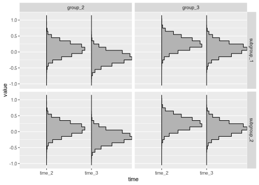
brm_plot_draws() is aware of any subgroup-specific marginal means.

brm_plot_draws(draws_subgroup$difference_group)

You can adjust visual aesthetics to compare subgroup levels side by side if subgroup level is the primary comparison of interest.

brm_plot_draws(
  draws_subgroup$difference_group,
  axis = "subgroup",
  facet = c("time", "group")
)

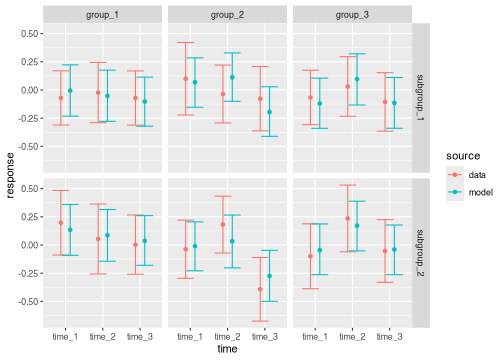
The following function call compares the subgroup model results against the subgroup data.

brm_plot_compare(
  data = summaries_data_subgroup,
  model = summaries_subgroup,
  marginal = "response"
)

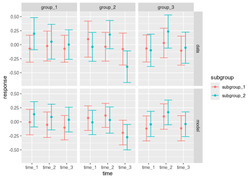
You can adjust plot aesthetics to view subgroup levels side by side as the primary comparison of interest.

brm_plot_compare(
  data = summaries_data_subgroup,
  model = summaries_subgroup,
  marginal = "response",
  compare = "subgroup",
  axis = "time",
  facet = c("group", "source")
)

We can also visually compare the treatment effects of a subgroup level against the marginal treatment effects of the reduced model.

brm_plot_compare(
  subgroup = filter(summaries_subgroup, subgroup == "subgroup_2"),
  reduced = summaries_reduced,
  marginal = "difference_group"
)

Please remember to filter on a single subgroup level. Otherwise, brm_plot_compare() throws an informative error to prevent overplotting.

brm_plot_compare(
  subgroup = summaries_subgroup,
  reduced = summaries_reduced,
  marginal = "difference_group"
)
#> Error:
#> ! brm_plot_compare() is omitting the subgroup variable because not all marginal summaries have it, but marginal summaries 'subgroup' have more than one subgroup level. Please either filter on a single subgroup level or make sure all supplied marginal summaries are subgroup-specific.

References

EMA (2019), Guideline on the investigation of subgroups in confirmatory clinical trials, European Medicines Agency; https://www.ema.europa.eu/en/investigation-subgroups-confirmatory-clinical-trials-scientific-guideline.

ICH (1998), “International council for harmonisation of technical requirements for pharmaceuticals for human use (ICH) E9 guideline. Statistical principles for clinical trials,” https://database.ich.org/sites/default/files/E9_Guideline.pdf.

Kent, D. M. (2023), “Overall average treatment effects from clinical trials, one-variable-at-a-time subgroup analyses and predictive approaches to heterogeneous treatment effects: Toward a more patient-centered evidence-based medicine,” Clin Trials, 20, 328–337.

Lipkovich, I., Dmitrienko, A., and B, R. (2017), “Tutorial in biostatistics: data-driven subgroup identification and analysis in clinical trials,” Stat Med, 36, 136–196.

Lipkovich, I., Svensson, D., Ratitch, B., and Dmitrienko, A. (2023), “Overview of modern approaches for identifying and evaluating heterogeneous treatment effects from clinical data,” Clin Trials, 20, 380–393.