Styling survival plots

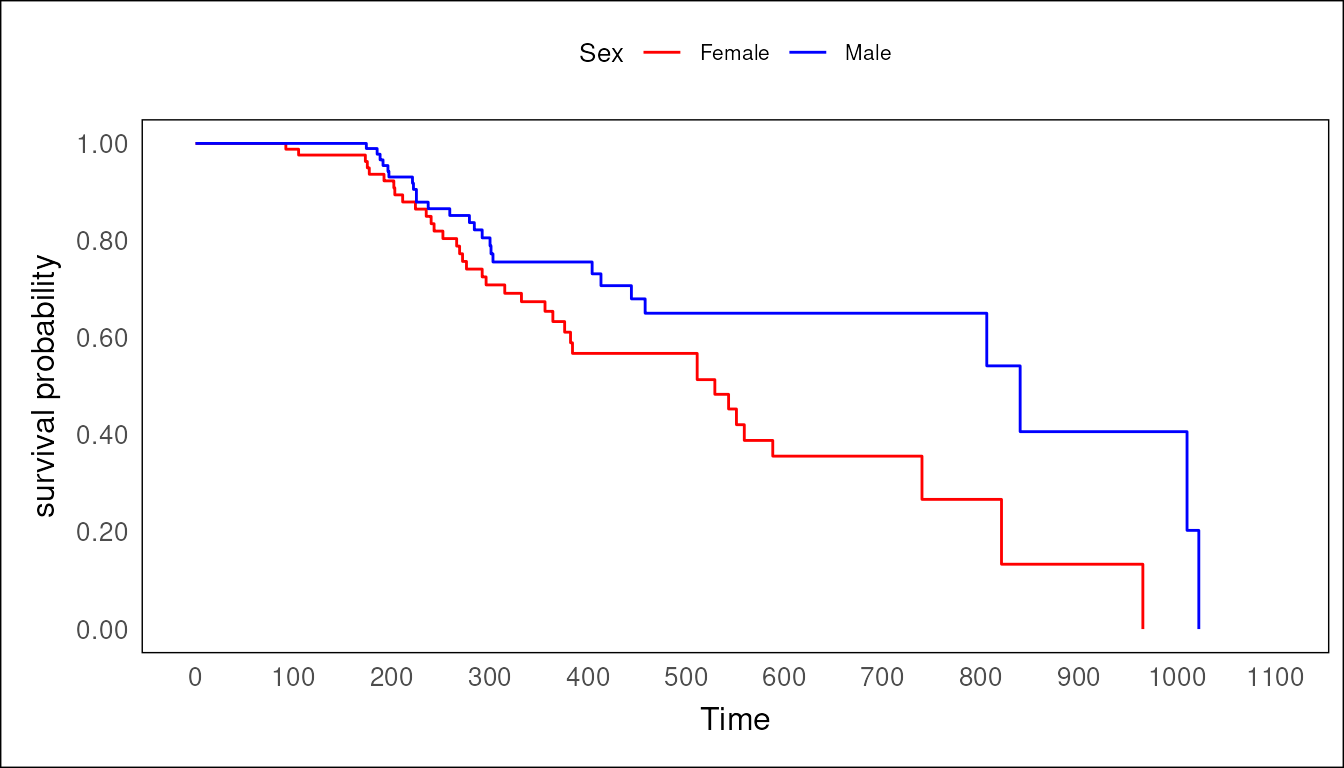
Introduction

library(visR)

This tutorial illustrates the usage of the styling function that visR provides. By default, visR::visr() does not apply any form of visual changes to the generated survival plots. Therefore, the default output looks like you would expect from a standard ggplot2::ggplot() plot. While the examples below visualize the results from estimate_KM(), these principles apply to competing risks cumulative incidence objects created with estimate_cuminc() as well.

Preparation of the data

In this example, we will work with patient data from NCCTG Lung Cancer dataset that is part of the survival package. This data is also used to demonstrate more functions of visR in another vignette. However, in this particular one, it will only be used to demonstrate the adjustments of the aesthetics.

Generation of a survfit object

lung_cohort <- survival::lung

lung_cohort <- lung_cohort %>%  
  dplyr::mutate(sex = as.factor(ifelse(sex == 1, "Male", "Female")))  %>%  
  dplyr::mutate(status = status - 1) %>%
  dplyr::rename(Age = "age", Sex = "sex", Status = "status", Days = "time") 

lung_suvival_object <- lung_cohort %>%
  visR::estimate_KM(strata = "Sex", CNSR = "Status", AVAL = "Days")
#> Warning: `estimate_KM()` was deprecated in visR 0.4.0.
#> ℹ Please use `ggsurvfit::ggsurvfit()` instead.
#> This warning is displayed once every 8 hours.
#> Call `lifecycle::last_lifecycle_warnings()` to see where this warning was
#> generated.

Styling

Plotting the generated survfit object without adjustments

p <- lung_suvival_object %>%
  visR::visr()
#> Warning: `visr.survfit()` was deprecated in visR 0.4.0.
#> ℹ Please use `ggsurvfit::ggsurvfit()` instead.
#> This warning is displayed once every 8 hours.
#> Call `lifecycle::last_lifecycle_warnings()` to see where this warning was
#> generated.
p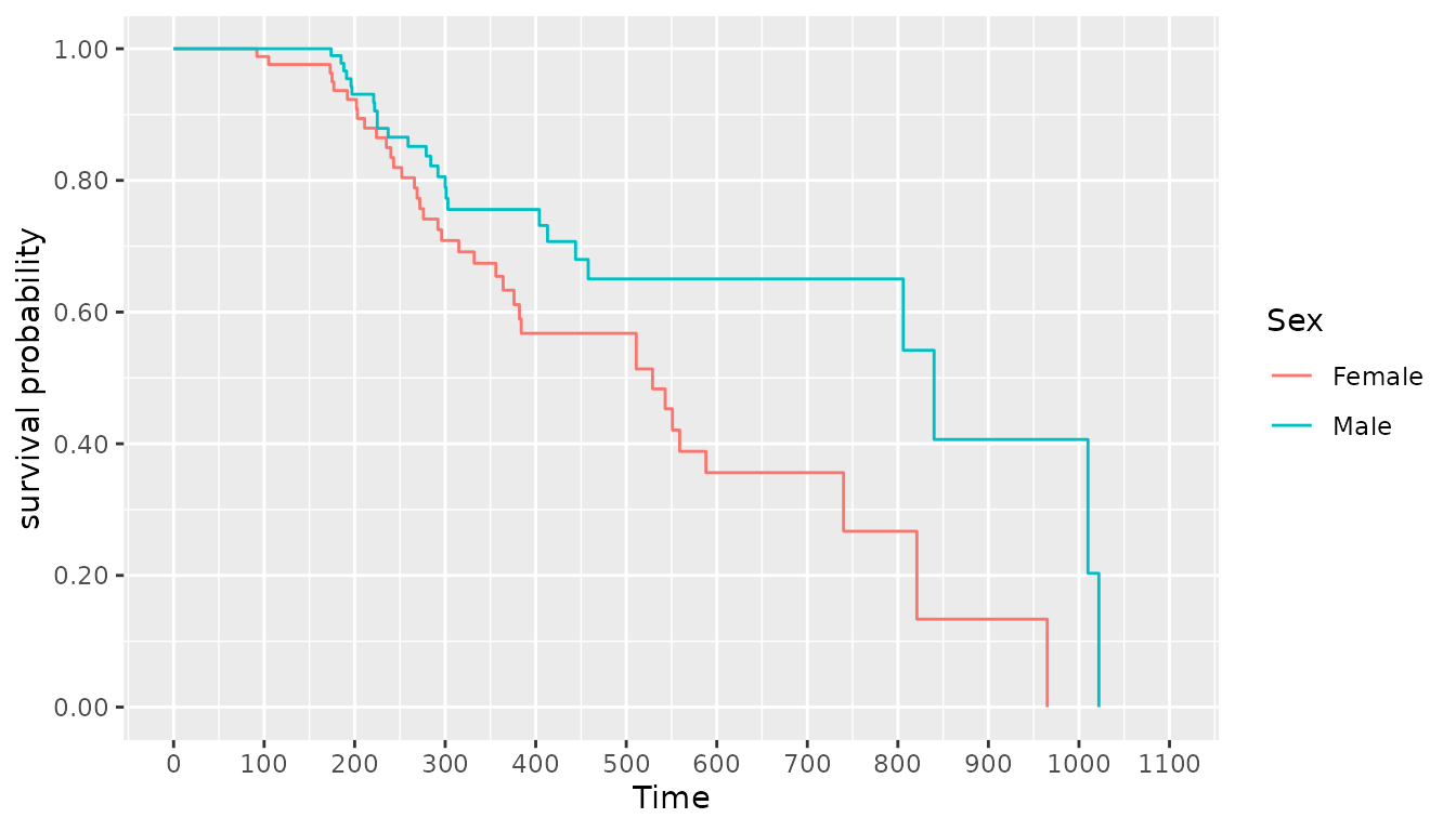

As we can, the plot shows the default ggplot2::theme_grey() style with a grey background, a visible grid and the default ggplot2 colours.

Using ggplot2 to style the plot

Since visR::visr() also generates a valid ggplot object as an output, we can use the conventional styling logic and options that ggplot2 provides, as shown below.

p +
  ggplot2::theme_bw() +
  ggplot2::theme(legend.position = "top") +
  ggplot2::scale_color_manual(values = c("red", "blue"))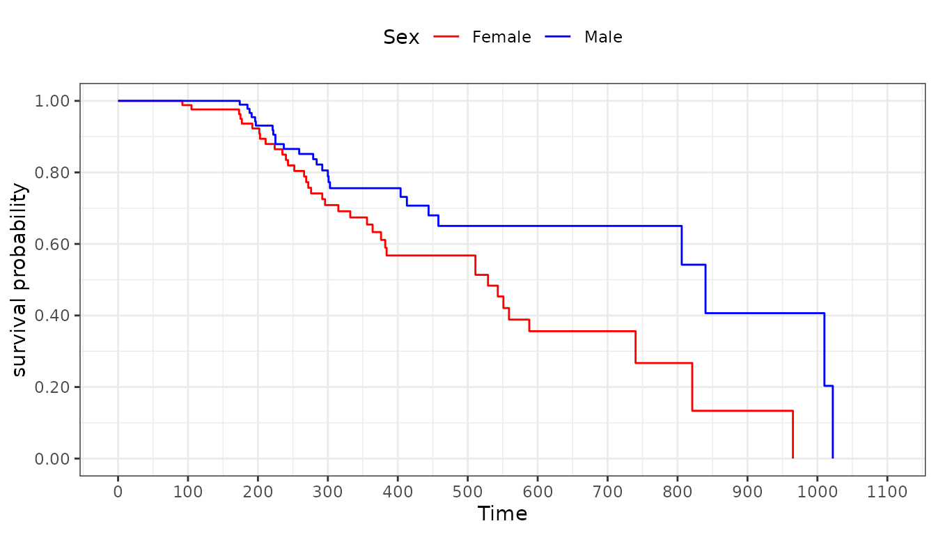

However, visR also provides functions to adjust common aesthetics more easily and with less code.

Using visR to style the plot

The most direct option to style plots generated through visR::visr() is by using the parameters that the function provides. Internally, parameters like the y-axis label are automatically deducted from the used function. The following example demonstrates the options exposed.

lung_suvival_object %>%
  visR::visr(x_label = "Time",
             y_label = NULL, # NULL (default) causes the label to be deducted from the used function
             x_ticks = seq(0, 1200, 200),
             y_ticks = seq(0, 100, 20),
             fun = "pct",
             legend_position = "top")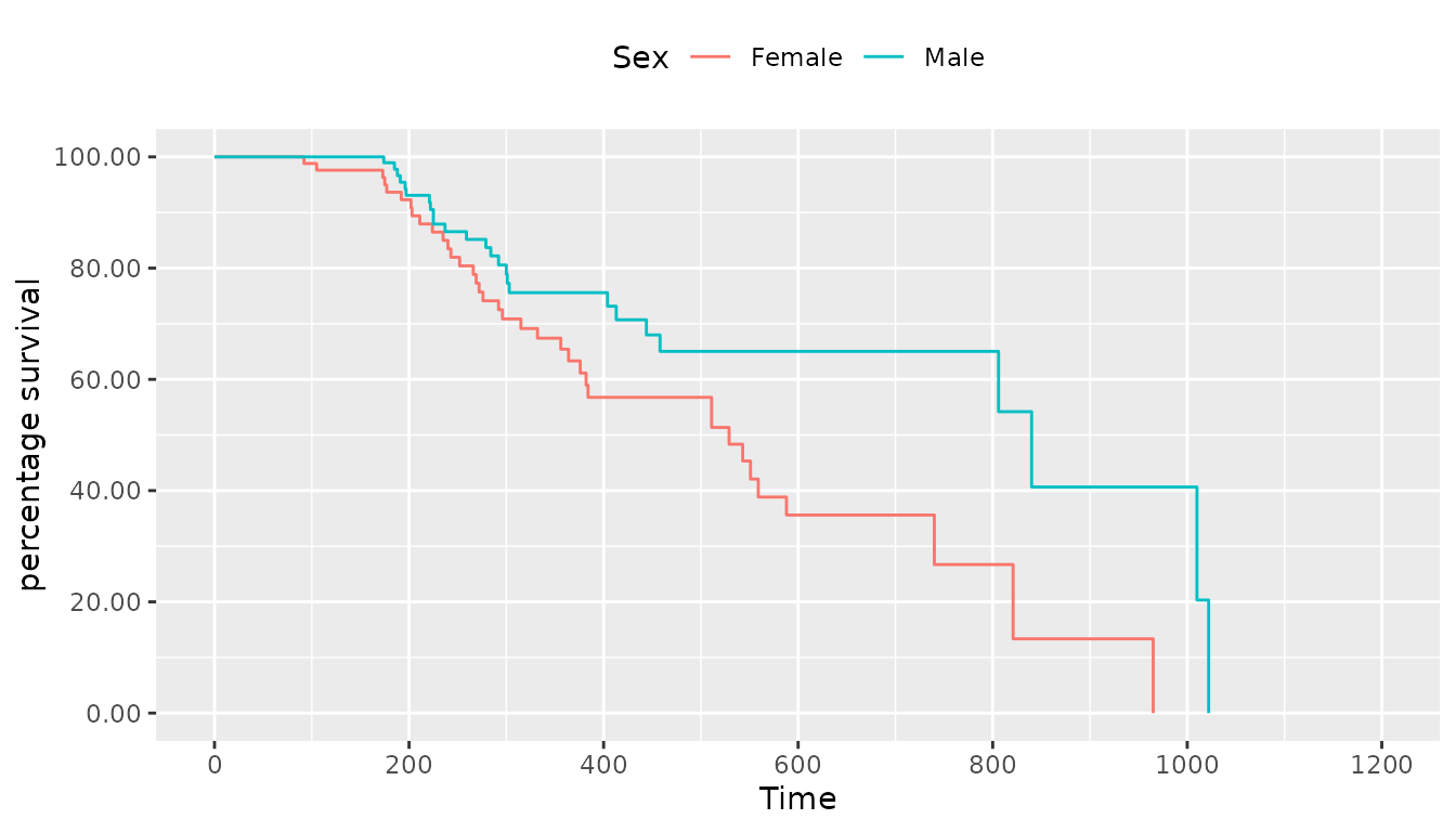 

However, these rather minimal adjustments usually don’t cover all the things a user wants to modify. Therefore, we provide two additional functions to adjust more aesthetics: visR::define_theme() and visR::apply_theme(). The first one provides an easy wrapper to create a nested list of list with styling options that is then applied to the plot by the second function.

New themes

Defining a visR_theme using visR::define_theme()

If no further options are provided to visR::define_theme(), it nonetheless returns a very minimal list of reasonable defaults.

visR::define_theme() 
#> $fontfamily
#> [1] "Helvetica"
#> 
#> $grid
#> [1] FALSE
#> 
#> $bg
#> [1] "transparent"
#> 
#> attr(,"class")
#> [1] "visR_theme" "list"

However, this function also takes several other styling options. The currently usable ones are displayed below. One particular use that we had in mind when writing this function was, that we wanted to have the option to define the different colours for the strata once and then to not have to worry about all of them being present.

theme <-
  visR::define_theme(
    strata = list(
      "Sex" = list("Female" = "red",
                   "Male" = "blue"),
      "ph.ecog" = list("0" = "cyan",
                       "1" = "purple",
                       "2" = "brown")
    ),
    fontsizes = list(
      "axis" = 12,
      "ticks" = 10,
      "legend_title" = 10,
      "legend_text" = 8
    ),
    fontfamily = "Helvetica",
    grid = list("major" = FALSE,
                "minor" = FALSE),
    #grid = TRUE/FALSE # <- can also be used instead of the named list above
    bg = "transparent",
    legend_position = "top"
  )

Apply styling using visR::apply_theme()

The visR::apply_theme() function exposes the user to two ways to style their plot. The most direct one would be to just apply the function to a plot without specifying any options. This applies several reasonable defaults to the plot.

lung_suvival_object %>%
  visR::visr() %>%
  visR::apply_theme()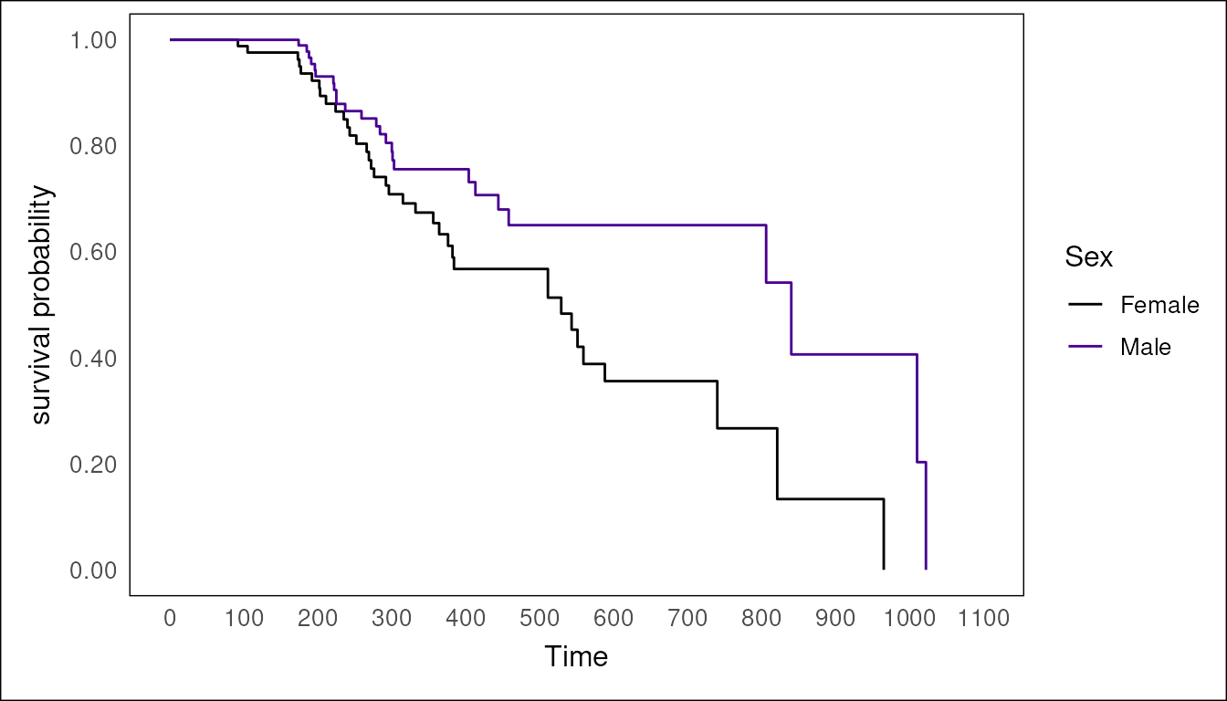

The second one would be to apply a nested list of lists to, ideally generated through visR::define_theme() to a plot. This serves the purpose to generate a detailed visR_theme object once and then apply it to one or several plots with a single line. These lists could then also be easily saved and shared. The usage of the theme generated above is shown below.

lung_suvival_object %>%
  visR::visr() %>%
  visR::apply_theme(theme)