Comparing {simaerep} and {gsm} Performance

Load

suppressPackageStartupMessages(library(tidyverse))
suppressPackageStartupMessages(library(knitr))
suppressPackageStartupMessages(library(furrr))
suppressPackageStartupMessages(library(future))
suppressPackageStartupMessages(library(simaerep))

plan(multisession, workers = 6)

Install {gsm}

devtools::install_github("Gilead-BioStats/gsm", ref = "main")

Introduction

The {gsm} R package provides a standardized Risk Based Quality Monitoring (RBQM) framework for clinical trials that pairs a flexible data pipeline with robust reports. It also uses Funnel Plots to flag outliers which provide broader tolerance limits for sites with low exposure and narrower limits for sites with higher exposure. This method is different to the event rate based limits we have used in previous heuristics to measure {simaerep} performance. Funnel plots are discussed in greater detail by Zink et al. 2018

One of the draw backs of using funnel plots for flagging is that they assume that the AE rate remains constant over the course of the study.

Prepare Data

Load Portfolio Configurations

We have prepared a snapshot of the AE reporting configuration of our current portfolio. For each study we have also measured a visit-specific AE rate which allows us to generate a synthetic portfolio with flexible AE rates across a study.

df_config <- readr::read_csv("ae_conf_20240220.csv")
df_ae_rates <- readr::read_csv("ae_rates_20240220.csv")

df_config %>%
  head(25) %>%
  knitr::kable()

study_id	ae_per_visit_mean	site_number	max_visit_sd	max_visit_mean	n_pat
0001	0.2973806	4746	3.5355339	16.50000	2
0001	0.2973806	4747	0.7071068	27.50000	2
0001	0.2973806	4750	0.5000000	19.25000	4
0001	0.2973806	4815	8.3765546	22.16667	6
0001	0.2973806	4816	0.0000000	27.00000	1
0001	0.2973806	4817	0.0000000	31.00000	1
0001	0.2973806	4818	0.0000000	30.00000	1
0001	0.2973806	4891	2.3804761	22.00000	7
0001	0.2973806	4893	0.0000000	20.00000	2
0001	0.2973806	4932	1.0954451	26.80000	5
0001	0.2973806	4941	1.7320508	27.00000	3
0001	0.2973806	4942	1.4142136	25.00000	2
0001	0.2973806	4943	0.0000000	25.00000	1
0001	0.2973806	4966	0.0000000	18.00000	1
0001	0.2973806	4967	0.8164966	18.00000	4
0001	0.2973806	4968	0.0000000	24.00000	1
0001	0.2973806	4969	1.5275252	21.33333	3
0001	0.2973806	4984	1.7078251	30.75000	4
0001	0.2973806	4985	8.9087972	21.16667	6
0001	0.2973806	4986	0.5773503	20.33333	3
0001	0.2973806	4988	1.4142136	19.00000	2
0001	0.2973806	5079	2.1602469	23.00000	4
0001	0.2973806	5080	0.0000000	23.00000	1
0001	0.2973806	5081	0.0000000	23.00000	1
0001	0.2973806	5082	1.4142136	22.00000	2

df_ae_rates %>%
  head(25) %>%
  knitr::kable()

study_id	cum_visit	ae_rate	n_pat
0001	1	0.017699	113
0001	2	0.088496	113
0001	3	0.230088	113
0001	4	0.223214	112
0001	5	0.187500	112
0001	6	0.196429	112
0001	7	0.396396	111
0001	8	0.207207	111
0001	9	0.216216	111
0001	10	0.315315	111
0001	11	0.263636	110
0001	12	0.318182	110
0001	13	0.345455	110
0001	14	0.379630	108
0001	15	0.401869	107
0001	16	0.485981	107
0001	17	0.383178	107
0001	18	0.396226	106
0001	19	0.370000	100
0001	20	0.439560	91
0001	21	0.369863	73
0001	22	0.370968	62
0001	23	0.345455	55
0001	24	0.446809	47
0001	25	0.292683	41

Simulate Portfolio

We generate two synthetic portfolios with no AE under-reporting sites. One portfolio with a fixed AE rate for all visits and another one with a flexible visit-specific AE rate.

df_portf_fix <- sim_test_data_portfolio(df_config, parallel = TRUE, progress = TRUE)

df_portf_fix %>%
  head(25) %>%
  knitr::kable()

study_id	ae_per_visit_mean	site_number	max_visit_sd	max_visit_mean	patnum	visit	n_ae
0001	0.2973806	4746	3.535534	16.5	0001	1	2
0001	0.2973806	4746	3.535534	16.5	0001	2	2
0001	0.2973806	4746	3.535534	16.5	0001	3	2
0001	0.2973806	4746	3.535534	16.5	0001	4	2
0001	0.2973806	4746	3.535534	16.5	0001	5	2
0001	0.2973806	4746	3.535534	16.5	0001	6	2
0001	0.2973806	4746	3.535534	16.5	0001	7	4
0001	0.2973806	4746	3.535534	16.5	0001	8	5
0001	0.2973806	4746	3.535534	16.5	0001	9	6
0001	0.2973806	4746	3.535534	16.5	0001	10	6
0001	0.2973806	4746	3.535534	16.5	0001	11	6
0001	0.2973806	4746	3.535534	16.5	0001	12	6
0001	0.2973806	4746	3.535534	16.5	0001	13	8
0001	0.2973806	4746	3.535534	16.5	0002	1	0
0001	0.2973806	4746	3.535534	16.5	0002	2	0
0001	0.2973806	4746	3.535534	16.5	0002	3	0
0001	0.2973806	4746	3.535534	16.5	0002	4	0
0001	0.2973806	4746	3.535534	16.5	0002	5	0
0001	0.2973806	4746	3.535534	16.5	0002	6	0
0001	0.2973806	4746	3.535534	16.5	0002	7	0
0001	0.2973806	4746	3.535534	16.5	0002	8	0
0001	0.2973806	4746	3.535534	16.5	0002	9	1
0001	0.2973806	4746	3.535534	16.5	0002	10	1
0001	0.2973806	4746	3.535534	16.5	0002	11	1
0001	0.2973806	4746	3.535534	16.5	0002	12	1

df_portf_flex <- sim_test_data_portfolio(df_config, df_ae_rates = df_ae_rates, parallel = TRUE, progress = TRUE)

Compare AE rates

Next we confirm the different AE rates in our two synthetic portfolios.

df_rate_fix <- df_portf_fix %>%
  mutate(ae_rate = coalesce(n_ae - lag(n_ae), n_ae), .by = c("study_id", "patnum")) %>%
  summarise(ae_rate = mean(ae_rate), .by = c("study_id", "visit")) %>%
  mutate(rate = "fix")


df_rate_flex <- df_portf_flex %>%
  mutate(ae_rate = coalesce(n_ae - lag(n_ae), n_ae), .by = c("study_id", "patnum")) %>%
  summarise(ae_rate = mean(ae_rate), .by = c("study_id", "visit")) %>%
  mutate(rate = "flex")

bind_rows(df_rate_flex, df_rate_fix) %>%
  ggplot(aes(visit, ae_rate)) +
    geom_line(aes(group = study_id), alpha = 0.2) +
    geom_smooth() +
    facet_wrap(~ rate) +
    labs(title = "Average AE rates per Study")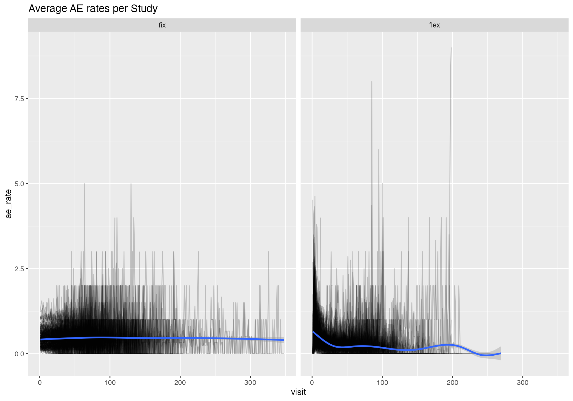

bind_rows(df_rate_flex, df_rate_fix) %>%
  filter(dense_rank(study_id) <= 16) %>%
  ggplot(aes(visit, ae_rate)) +
    geom_line(aes(group = rate, color = rate)) +
    facet_wrap(~ study_id, scales = "free") +
    labs(title = "Average AE rates for Selected Studies")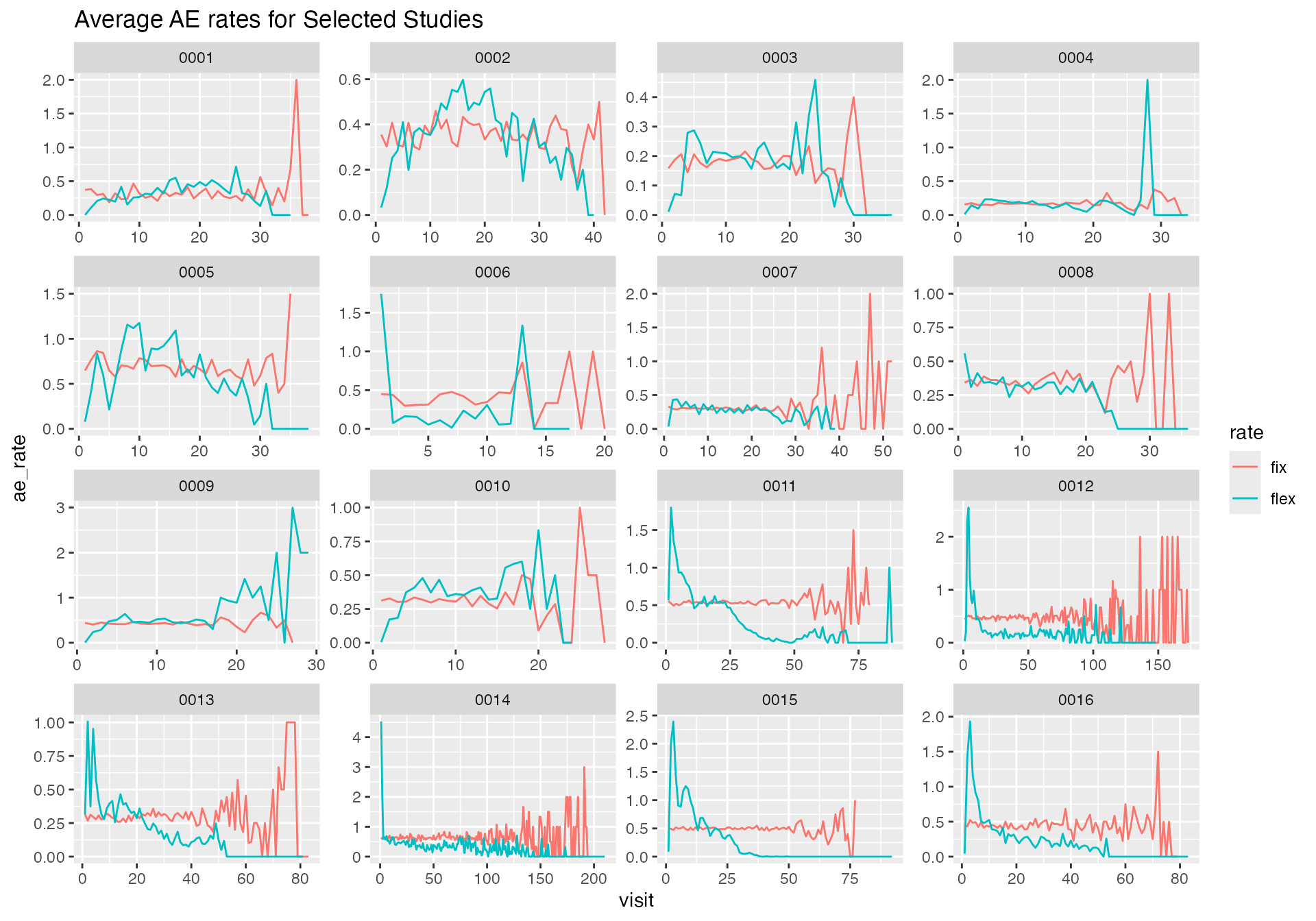

We can confirm that the AE rates in the “flexible” portfolio are not constant. Moreover we see that the AE rate profile is very unique for each study.

Apply {gsm}

Example

Here we demonstrate how to use the {gsm} package on our simulated portfolios.

get_SUBJ <- function(df_portf) {
  df_portf %>%
    select(study_id, siteid = site_number, subjid = patnum, timeonstudy = visit) %>%
    summarise(timeonstudy = max(timeonstudy), .by = c(study_id, siteid, subjid)) %>%
    group_by(study_id) %>%
    nest()
}


get_AE <- function(df_portf) {
  df_portf_fix %>%
    select(study_id, subjid = patnum, n_ae) %>%
    summarise(n_ae = max(n_ae), .by = c(study_id, subjid)) %>%
    filter(n_ae > 0) %>%
    mutate(n_ae = map(n_ae, ~ tibble(n = seq(1, .)), .progress = TRUE)) %>%
    unnest(n_ae) %>%
    select(- n) %>%
    group_by(study_id) %>%
    nest()
}

dfSUBJ_fix <- get_SUBJ(df_portf_fix)
dfAE_fix <- get_AE(df_portf_fix)

dfInput <- gsm::AE_Map_Raw(list(dfSUBJ = dfSUBJ_fix$data[[1]], dfAE = dfAE_fix$data[[1]]))
dfInput

## # A tibble: 113 × 5
##    SubjectID SiteID Exposure Count  Rate
##    <chr>     <chr>     <int> <int> <dbl>
##  1 0001      4746         13     8 0.615
##  2 0002      4746         20     5 0.25 
##  3 0003      4747         27    10 0.370
##  4 0004      4747         26     9 0.346
##  5 0005      4750         19     7 0.368
##  6 0006      4750         19     4 0.211
##  7 0007      4750         20     3 0.15 
##  8 0008      4750         19     3 0.158
##  9 0009      4815          9     4 0.444
## 10 0010      4815         32    12 0.375
## # ℹ 103 more rows

dfTransformed <- gsm::Transform_Rate(
  dfInput,
  strNumeratorCol = "Count",
  strDenominatorCol = "Exposure"
  )
dfTransformed

## # A tibble: 44 × 4
##    GroupID Numerator Denominator Metric
##    <chr>       <int>       <int>  <dbl>
##  1 4746           13          33  0.394
##  2 4747           19          53  0.358
##  3 4750           17          77  0.221
##  4 4815           50         147  0.340
##  5 4816            6          27  0.222
##  6 4817           13          31  0.419
##  7 4818            7          30  0.233
##  8 4891           46         146  0.315
##  9 4893           14          40  0.35 
## 10 4932           42         135  0.311
## # ℹ 34 more rows

dfAnalyzed <- gsm::Analyze_NormalApprox(dfTransformed)
dfAnalyzed

## # A tibble: 44 × 7
##    GroupID Numerator Denominator Metric OverallMetric Factor  Score
##    <chr>       <int>       <int>  <dbl>         <dbl>  <dbl>  <dbl>
##  1 5084            2          21 0.0952         0.307   1.10 -2.00 
##  2 5168            8          44 0.182          0.307   1.10 -1.71 
##  3 4750           17          77 0.221          0.307   1.10 -1.56 
##  4 5080            4          23 0.174          0.307   1.10 -1.32 
##  5 5081            4          23 0.174          0.307   1.10 -1.32 
##  6 5111            6          31 0.194          0.307   1.10 -1.30 
##  7 5082           10          45 0.222          0.307   1.10 -1.17 
##  8 5311            4          20 0.2            0.307   1.10 -0.987
##  9 4942           12          50 0.24           0.307   1.10 -0.976
## 10 5273           10          42 0.238          0.307   1.10 -0.920
## # ℹ 34 more rows

dfFlagged <- gsm::Flag_NormalApprox(dfAnalyzed, vThreshold = c(-3, -2, 2, 3))
dfFlagged

## # A tibble: 44 × 8
##    GroupID Numerator Denominator Metric OverallMetric Factor  Score  Flag
##    <chr>       <int>       <int>  <dbl>         <dbl>  <dbl>  <dbl> <dbl>
##  1 5084            2          21 0.0952         0.307   1.10 -2.00     -1
##  2 5168            8          44 0.182          0.307   1.10 -1.71      0
##  3 4750           17          77 0.221          0.307   1.10 -1.56      0
##  4 5080            4          23 0.174          0.307   1.10 -1.32      0
##  5 5081            4          23 0.174          0.307   1.10 -1.32      0
##  6 5111            6          31 0.194          0.307   1.10 -1.30      0
##  7 5082           10          45 0.222          0.307   1.10 -1.17      0
##  8 5311            4          20 0.2            0.307   1.10 -0.987     0
##  9 4942           12          50 0.24           0.307   1.10 -0.976     0
## 10 5273           10          42 0.238          0.307   1.10 -0.920     0
## # ℹ 34 more rows

dfSummary <- gsm::Summarize(dfFlagged)
dfSummary

## # A tibble: 44 × 6
##    GroupID Numerator Denominator Metric  Score  Flag
##    <chr>       <int>       <int>  <dbl>  <dbl> <dbl>
##  1 5084            2          21 0.0952 -2.00     -1
##  2 5308           26          61 0.426   1.93      0
##  3 4817           13          31 0.419   1.30      0
##  4 4968           10          24 0.417   1.11      0
##  5 5224           10          24 0.417   1.11      0
##  6 4943           10          25 0.4     0.965     0
##  7 4746           13          33 0.394   1.04      0
##  8 5135            7          18 0.389   0.721     0
##  9 4988           14          37 0.378   0.902     0
## 10 5166           35          93 0.376   1.39      0
## # ℹ 34 more rows

dfBounds <- gsm::Analyze_NormalApprox_PredictBounds(dfTransformed, vThreshold = c(-3, -2, 2, 3))
dfBounds

## # A tibble: 1,258 × 5
##    Threshold Denominator LogDenominator Numerator   Metric
##        <dbl>       <dbl>          <dbl>     <dbl>    <dbl>
##  1        -3        22.4           3.11   0.00938 0.000419
##  2        -3        23.2           3.14   0.123   0.00533 
##  3        -3        23.9           3.17   0.239   0.0100  
##  4        -3        24.6           3.20   0.356   0.0145  
##  5        -3        25.4           3.23   0.475   0.0187  
##  6        -3        26.1           3.26   0.596   0.0228  
##  7        -3        26.8           3.29   0.718   0.0268  
##  8        -3        27.6           3.32   0.841   0.0305  
##  9        -3        28.3           3.34   0.966   0.0341  
## 10        -3        29.0           3.37   1.09    0.0376  
## # ℹ 1,248 more rows

chart <- gsm::Visualize_Scatter(dfFlagged, dfBounds)
chart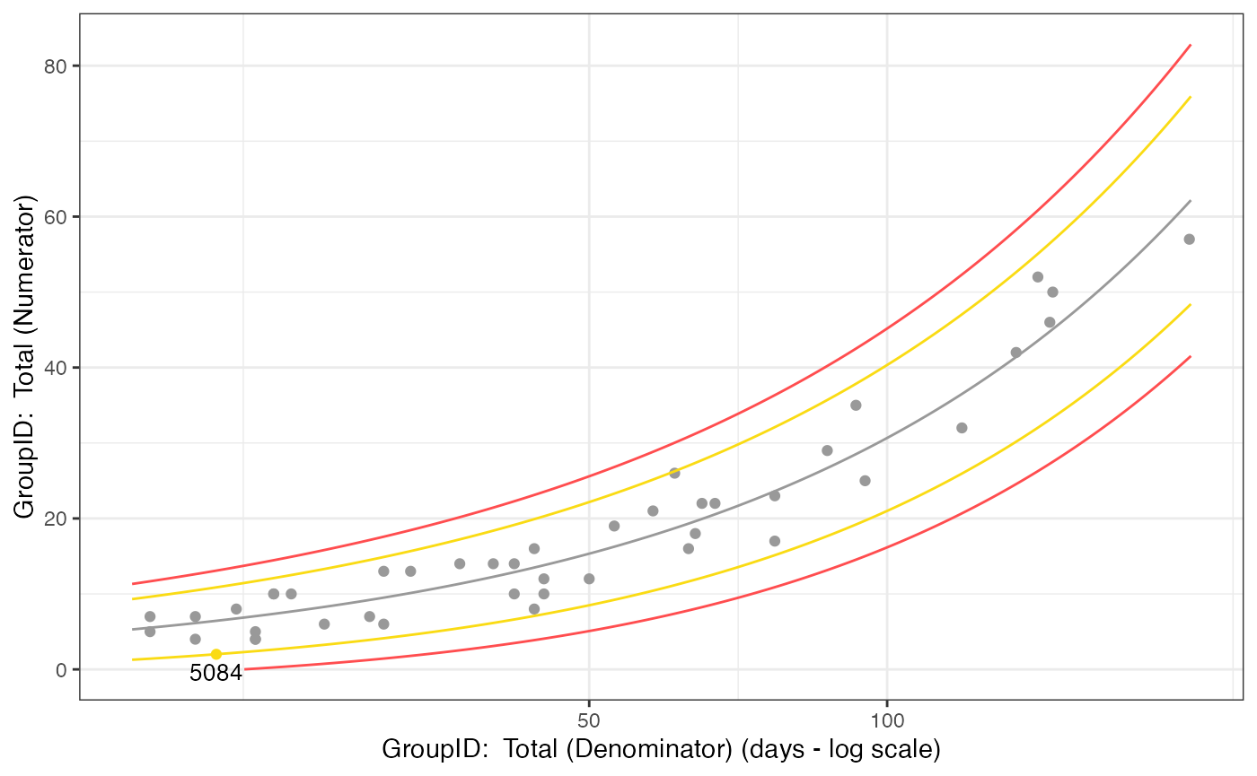

Simulate UR

We write a function that removes a given ratio of AEs from one site in the data set and returns its z-score.

sim_site_ur_gsm <- function(site, ur_rate, dfTransformed) {
  dfTransformed <- dfTransformed %>%
    mutate(
      Numerator = ifelse(GroupID == site, Numerator * (1 - ur_rate), Numerator),
      Metric = Numerator / Denominator
    )
  
  gsm::Analyze_NormalApprox(dfTransformed) %>%
    filter(GroupID == site) %>%
    pull(Score)
}

sim_site_ur_gsm("4747", ur_rate = 0.75, dfTransformed)

## [1] -2.88228

We write another function that systematically applies this sim_site_ur_gsm across all sites in all studies across a range of under-reporting ratios.

sim_ur_gsm <- function(dfSUBJ, dfAE) {
  dfSUBJ %>%
    inner_join(dfAE, by = "study_id") %>%
    ungroup() %>%
    mutate(
      trans = map2(data.x, data.y, ~ gsm::AE_Map_Raw(list(dfSUBJ = .x, dfAE = .y))),
      trans = map(trans, ~ gsm::Transform_Rate(., strNumeratorCol = "Count", strDenominatorCol = "Exposure")),
      sites = map(data.x, ~ distinct(., siteid))
    ) %>%
    select(- starts_with("data.")) %>%
    unnest(sites) %>%
    mutate(ur = list(tibble(ur_rate = c(0, 0.1, 0.25, 0.5, 0.75, 1)))) %>%
    unnest(ur) %>%
    mutate(
      score = pmap_dbl(list(siteid, ur_rate, trans), sim_site_ur_gsm, .progress = TRUE)
    )
}

df_sim_gsm_fix <- sim_ur_gsm(dfSUBJ_fix, dfAE_fix)

## Warning: There were 3095 warnings in `mutate()`.
## The first warning was:
## ℹ In argument: `z_i = ifelse(...)`.
## Caused by warning:
## ! There was 1 warning in `mutate()`.
## ℹ In argument: `z_0 = ifelse(...)`.
## Caused by warning in `sqrt()`:
## ! NaNs produced
## ℹ Run `dplyr::last_dplyr_warnings()` to see the 3094 remaining warnings.

df_sim_gsm_fix

## # A tibble: 129,966 × 5
##    study_id trans             siteid ur_rate  score
##    <chr>    <list>            <chr>    <dbl>  <dbl>
##  1 0001     <tibble [44 × 4]> 4746      0     1.04 
##  2 0001     <tibble [44 × 4]> 4746      0.1   0.580
##  3 0001     <tibble [44 × 4]> 4746      0.25 -0.120
##  4 0001     <tibble [44 × 4]> 4746      0.5  -1.27 
##  5 0001     <tibble [44 × 4]> 4746      0.75 -2.30 
##  6 0001     <tibble [44 × 4]> 4746      1    -3.18 
##  7 0001     <tibble [44 × 4]> 4747      0     0.780
##  8 0001     <tibble [44 × 4]> 4747      0.1   0.253
##  9 0001     <tibble [44 × 4]> 4747      0.25 -0.544
## 10 0001     <tibble [44 × 4]> 4747      0.5  -1.80 
## # ℹ 129,956 more rows

We repeat the same steps for the portfolio with the flexible AE rates.

dfSUBJ_flex <- get_SUBJ(df_portf_flex)
dfAE_flex<- get_AE(df_portf_flex)


df_sim_gsm_flex <- sim_ur_gsm(dfSUBJ_flex, dfAE_flex)

## Warning: There were 3004 warnings in `mutate()`.
## The first warning was:
## ℹ In argument: `z_i = ifelse(...)`.
## Caused by warning:
## ! There was 1 warning in `mutate()`.
## ℹ In argument: `z_0 = ifelse(...)`.
## Caused by warning in `sqrt()`:
## ! NaNs produced
## ℹ Run `dplyr::last_dplyr_warnings()` to see the 3003 remaining warnings.

UR {simaerep}

We simulate under-reporting for both portfolios using {simaerep}

df_sim_simaerep_fix <- sim_ur_scenarios(
   df_portf_fix,
   extra_ur_sites = 0,
   ur_rate = c(0, 0.1, 0.25, 0.5, 0.75, 1),
   parallel = TRUE,
   poisson = TRUE,
   prob_lower = TRUE,
   progress = TRUE
)

df_sim_simaerep_flex <- sim_ur_scenarios(
   df_portf_flex,
   extra_ur_sites = 0,
   ur_rate = c(0, 0.1, 0.25, 0.5, 0.75, 1),
   parallel = TRUE,
   poisson = TRUE,
   prob_lower = TRUE,
   progress = TRUE
)

Evaluate

Combine Results

df_sim_gsm_fix$ae_rate <- "AE rate: fix"
df_sim_gsm_flex$ae_rate <- "AE rate: flexible"
df_sim_simaerep_fix$ae_rate <- "AE rate: fix"
df_sim_simaerep_flex$ae_rate <- "AE rate: flexible"

df_sim_thresh2 <- bind_rows(df_sim_gsm_fix, df_sim_gsm_flex) %>%
  mutate(
    is_ur = score <= -2,
    type = "{gsm} - thresh: -2",
    site_number = siteid
  ) %>%
  select(type, ae_rate, study_id, site_number, ur_rate, is_ur, score)


df_sim_simaerep_threshp95 <-  bind_rows(df_sim_simaerep_fix, df_sim_simaerep_flex) %>%
  mutate(
    is_ur = prob_low_prob_ur >= 0.95,
    type = "{simaerep} - thresh: 0.95"
  ) %>%
  select(type, ae_rate, study_id, site_number, ur_rate, is_ur, score = prob_low_prob_ur)


df_eval <- bind_rows(
  df_sim_thresh2,
  df_sim_simaerep_threshp95,
)

Aggregate

get_prop_test_ci95 <- function(..., ix) {
  
  stopifnot(ix %in% c(1, 2))
  
  tryCatch(
    prop.test(...)$conf.int[ix],
    error = function(cnd) c(NA, NA)[ix]
  )
}

aggr_results <- function(df_eval) {

df_perf <- df_eval %>%
  summarise(
    n = n(),
    .by = c(type, ae_rate, ur_rate, is_ur)
  ) %>%
  pivot_wider(
    names_from = is_ur,
    values_from = n,
    names_prefix = "is_ur_",
    values_fill = 0
  ) %>%
  mutate(
    n_sites = is_ur_TRUE + is_ur_FALSE + is_ur_NA,
    ratio = is_ur_TRUE / n_sites,
    ratio_type = ifelse(ur_rate == 0, "fpr", "tpr"),
    ci95_low = map2_dbl(is_ur_TRUE, n_sites, ~ get_prop_test_ci95(.x, .y, ix = 1)),
    ci95_high = map2_dbl(is_ur_TRUE, n_sites, ~ get_prop_test_ci95(.x, .y, ix = 2))
  )
}

df_perf <- aggr_results(df_eval)

Results

Table

df_perf %>%
  knitr::kable(digits = 3)

type	ae_rate	ur_rate	is_ur_FALSE	is_ur_TRUE	is_ur_NA	n_sites	ratio	ratio_type	ci95_low	ci95_high
{gsm} - thresh: -2	AE rate: fix	0.00	20823	306	532	21661	0.014	fpr	0.013	0.016
{gsm} - thresh: -2	AE rate: fix	0.10	19868	1262	531	21661	0.058	tpr	0.055	0.061
{gsm} - thresh: -2	AE rate: fix	0.25	15878	5258	525	21661	0.243	tpr	0.237	0.249
{gsm} - thresh: -2	AE rate: fix	0.50	9273	11876	512	21661	0.548	tpr	0.542	0.555
{gsm} - thresh: -2	AE rate: fix	0.75	5263	15895	503	21661	0.734	tpr	0.728	0.740
{gsm} - thresh: -2	AE rate: fix	1.00	3027	18142	492	21661	0.838	tpr	0.833	0.842
{gsm} - thresh: -2	AE rate: flexible	0.00	20886	254	521	21661	0.012	fpr	0.010	0.013
{gsm} - thresh: -2	AE rate: flexible	0.10	20677	465	519	21661	0.021	tpr	0.020	0.024
{gsm} - thresh: -2	AE rate: flexible	0.25	19703	1444	514	21661	0.067	tpr	0.063	0.070
{gsm} - thresh: -2	AE rate: flexible	0.50	16318	4848	495	21661	0.224	tpr	0.218	0.229
{gsm} - thresh: -2	AE rate: flexible	0.75	12281	8896	484	21661	0.411	tpr	0.404	0.417
{gsm} - thresh: -2	AE rate: flexible	1.00	8774	12416	471	21661	0.573	tpr	0.567	0.580
{simaerep} - thresh: 0.95	AE rate: fix	0.00	21363	298	0	21661	0.014	fpr	0.012	0.015
{simaerep} - thresh: 0.95	AE rate: fix	0.10	20406	1255	0	21661	0.058	tpr	0.055	0.061
{simaerep} - thresh: 0.95	AE rate: fix	0.25	17187	4474	0	21661	0.207	tpr	0.201	0.212
{simaerep} - thresh: 0.95	AE rate: fix	0.50	10660	11001	0	21661	0.508	tpr	0.501	0.515
{simaerep} - thresh: 0.95	AE rate: fix	0.75	5874	15787	0	21661	0.729	tpr	0.723	0.735
{simaerep} - thresh: 0.95	AE rate: fix	1.00	4043	17618	0	21661	0.813	tpr	0.808	0.819
{simaerep} - thresh: 0.95	AE rate: flexible	0.00	21356	305	0	21661	0.014	fpr	0.013	0.016
{simaerep} - thresh: 0.95	AE rate: flexible	0.10	20267	1394	0	21661	0.064	tpr	0.061	0.068
{simaerep} - thresh: 0.95	AE rate: flexible	0.25	16694	4967	0	21661	0.229	tpr	0.224	0.235
{simaerep} - thresh: 0.95	AE rate: flexible	0.50	9975	11686	0	21661	0.539	tpr	0.533	0.546
{simaerep} - thresh: 0.95	AE rate: flexible	0.75	5404	16257	0	21661	0.751	tpr	0.745	0.756
{simaerep} - thresh: 0.95	AE rate: flexible	1.00	3707	17954	0	21661	0.829	tpr	0.824	0.834

Plot Performance Metrics

• {gsm} has better performance than {simaerep} when the AE rate is fixed, while {simaerep} greatly outperforms {gsm} when the AE rate is flexible and mimics the AE rates encountered in real study data sets.

plot_perf <- function(df_perf) {

  df_perf %>%
    mutate(ur_rate = paste0("under-reporting rate: ",  ur_rate, " - ", ratio_type),
           ur_rate = ifelse(str_detect(ur_rate, "fpr"), "fpr", ur_rate)) %>%
    group_by(ur_rate) %>%
    ggplot(aes(type, ratio)) +
      geom_errorbar(aes(ymin = ci95_low, ymax = ci95_high, color = type), linewidth = 1) +
      facet_grid(ur_rate ~ ae_rate) +
      coord_flip() +
      theme(legend.position = "bottom") +
      labs(
        x = "",
        y = "CI95 Performance Ratio", 
        title = "{simaerep} vs {gsm} Performance"
      ) +
      scale_color_manual(values = c("#5491CC", "#F46626"))
}

plot_perf(df_perf)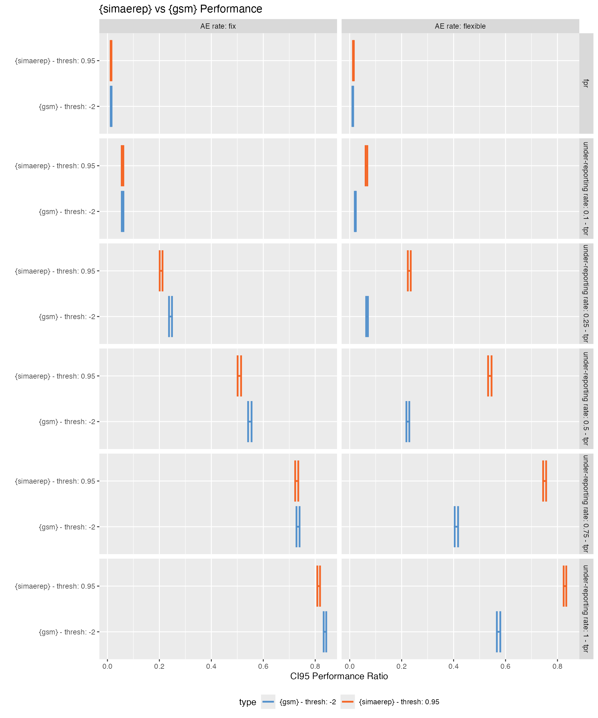

plan(sequential)