Address Usability Limits of Bootstrap Method
Source:vignettes/usability_limits.Rmd
usability_limits.RmdIntroduction
As we already mentioned in the introduction bootstrap resampling comes at a price. We need a good proportion of sites that are compliant and are not under-reporting AEs. Otherwise the patient pool we draw from will be tainted. Also, in general for count data, negative deviations from overall small integer values (3 or less) are hard to detect. Here we will assess the usability limits of the bootstrap resampling method by applying it to different simulated scenarios.
Parameter Grid
We start by defining a parameter grid.
Fixed Parameters:
- n_pat: 1000
- n_sites: 100
- max_visit_mean: 20
- max_visit_sd: 4
Variable Parameters:
- ae_visit: 0.05 - 2
- frac_sites_wit_ur: 0.05 - 0.75
- ur_rate: 0.05 - 1
set.seed(1)

df_grid <- tibble( ae_per_visit_mean = seq(0.05, 2, length.out = 10)) %>%
  mutate(frac_site_with_ur = list(seq(0.05, 0.75, length.out = 10))) %>%
  unnest(frac_site_with_ur) %>%
  mutate(ur_rate = list(seq(0.05, 1, length.out = 10)) ) %>%
  unnest(ur_rate)

df_grid
## # A tibble: 1,000 × 3
## ae_per_visit_mean frac_site_with_ur ur_rate
## <dbl> <dbl> <dbl>
## 1 0.05 0.05 0.05
## 2 0.05 0.05 0.156
## 3 0.05 0.05 0.261
## 4 0.05 0.05 0.367
## 5 0.05 0.05 0.472
## 6 0.05 0.05 0.578
## 7 0.05 0.05 0.683
## 8 0.05 0.05 0.789
## 9 0.05 0.05 0.894
## 10 0.05 0.05 1
## # … with 990 more rowsApply
We use the furrr and
the future
package for multiprocessing. We proceed in applying all functions we
already introduced.
suppressWarnings(future::plan(multiprocess))Simulate Test Data
We iteratively apply sim_test_data_study() on the different parameter combination of the grid
df_grid <- df_grid %>%
  mutate(
    df_visit = furrr::future_pmap(
      list(am = ae_per_visit_mean,
           fr = frac_site_with_ur,
           ur = ur_rate),
      function(am, fr, ur) sim_test_data_study(n_pat = 1000,
                                               n_sites = 100,
                                               max_visit_mean = 20,
                                               max_visit_sd = 4,
                                               ae_per_visit_mean = am,
                                               frac_site_with_ur = fr,
                                               ur_rate = ur),
      .progress = FALSE,
      .options = furrr_options(seed = TRUE)
    )
  )

df_grid
## # A tibble: 1,000 × 4
## ae_per_visit_mean frac_site_with_ur ur_rate df_visit
## <dbl> <dbl> <dbl> <list>
## 1 0.05 0.05 0.05 <tibble [19,459 × 8]>
## 2 0.05 0.05 0.156 <tibble [19,631 × 8]>
## 3 0.05 0.05 0.261 <tibble [19,234 × 8]>
## 4 0.05 0.05 0.367 <tibble [19,523 × 8]>
## 5 0.05 0.05 0.472 <tibble [19,518 × 8]>
## 6 0.05 0.05 0.578 <tibble [19,545 × 8]>
## 7 0.05 0.05 0.683 <tibble [19,503 × 8]>
## 8 0.05 0.05 0.789 <tibble [19,351 × 8]>
## 9 0.05 0.05 0.894 <tibble [19,473 × 8]>
## 10 0.05 0.05 1 <tibble [19,489 × 8]>
## # … with 990 more rowsAggregate Test Data
We apply site_aggr() on the different simulated data sets.
df_grid <- df_grid %>%
  mutate(
    df_visit = map2(df_visit, row_number(),
                    function(x,y) mutate(x, study_id = paste("S", y))),
    df_site = furrr::future_map(df_visit,
                                site_aggr,
                                .progress = FALSE,
                                .options = furrr_options(seed = TRUE)
                                )
  )

df_grid
## # A tibble: 1,000 × 5
## ae_per_visit_mean frac_site_with_ur ur_rate df_visit df_site
## <dbl> <dbl> <dbl> <list> <list>
## 1 0.05 0.05 0.05 <tibble [19,459 × 9]> <tibble>
## 2 0.05 0.05 0.156 <tibble [19,631 × 9]> <tibble>
## 3 0.05 0.05 0.261 <tibble [19,234 × 9]> <tibble>
## 4 0.05 0.05 0.367 <tibble [19,523 × 9]> <tibble>
## 5 0.05 0.05 0.472 <tibble [19,518 × 9]> <tibble>
## 6 0.05 0.05 0.578 <tibble [19,545 × 9]> <tibble>
## 7 0.05 0.05 0.683 <tibble [19,503 × 9]> <tibble>
## 8 0.05 0.05 0.789 <tibble [19,351 × 9]> <tibble>
## 9 0.05 0.05 0.894 <tibble [19,473 × 9]> <tibble>
## 10 0.05 0.05 1 <tibble [19,489 × 9]> <tibble>
## # … with 990 more rowsSimulate Sites
We apply sim_sites() to to calculate the AE under-reporting probability.
df_grid <- df_grid %>%
  mutate( df_sim_sites = furrr::future_map2(df_site, df_visit,
                                            sim_sites,
                                            r = 1000,
                                            poisson_test = TRUE,
                                            prob_lower = TRUE,
                                            .progress = FALSE,
                                            .options = furrr_options(seed = TRUE)
                                            )
  )

df_grid
## # A tibble: 1,000 × 6
## ae_per_visit_mean frac_site_with_ur ur_rate df_visit df_site df_sim_sites
## <dbl> <dbl> <dbl> <list> <list> <list>
## 1 0.05 0.05 0.05 <tibble> <tibble> <tibble>
## 2 0.05 0.05 0.156 <tibble> <tibble> <tibble>
## 3 0.05 0.05 0.261 <tibble> <tibble> <tibble>
## 4 0.05 0.05 0.367 <tibble> <tibble> <tibble>
## 5 0.05 0.05 0.472 <tibble> <tibble> <tibble>
## 6 0.05 0.05 0.578 <tibble> <tibble> <tibble>
## 7 0.05 0.05 0.683 <tibble> <tibble> <tibble>
## 8 0.05 0.05 0.789 <tibble> <tibble> <tibble>
## 9 0.05 0.05 0.894 <tibble> <tibble> <tibble>
## 10 0.05 0.05 1 <tibble> <tibble> <tibble>
## # … with 990 more rowsEvaluate Sites
We apply eval_sites() to balance the bootstrapped probabilities by the expected number of false positives.
df_grid <- df_grid %>%
  mutate( df_eval = furrr::future_map(df_sim_sites,
                                      eval_sites,
                                      .progress = FALSE,
                                      .options = furrr_options(seed = TRUE)
                                      )
  )

df_grid
## # A tibble: 1,000 × 7
## ae_per_visit_mean frac_site_with_ur ur_rate df_visit df_site df_sim_sites
## <dbl> <dbl> <dbl> <list> <list> <list>
## 1 0.05 0.05 0.05 <tibble> <tibble> <tibble>
## 2 0.05 0.05 0.156 <tibble> <tibble> <tibble>
## 3 0.05 0.05 0.261 <tibble> <tibble> <tibble>
## 4 0.05 0.05 0.367 <tibble> <tibble> <tibble>
## 5 0.05 0.05 0.472 <tibble> <tibble> <tibble>
## 6 0.05 0.05 0.578 <tibble> <tibble> <tibble>
## 7 0.05 0.05 0.683 <tibble> <tibble> <tibble>
## 8 0.05 0.05 0.789 <tibble> <tibble> <tibble>
## 9 0.05 0.05 0.894 <tibble> <tibble> <tibble>
## 10 0.05 0.05 1 <tibble> <tibble> <tibble>
## # … with 990 more rows, and 1 more variable: df_eval <list>Get Metrics
Apart from calculating true and false positives rate for the final under-reporting probability we also calculate the same metrics for a couple of benchmark probabilities.
- p-values returned from
poisson.test() - and the probabilities and p-values before adjusting for the expected false positives
In all cases we use a 95% probability threshold.
get_metrics <- function(df_visit, df_eval, method) {

  if (method == "ptest") {
    prob_ur_adj = "pval_prob_ur"
    prob_ur_unadj = "pval"
  } else {
    prob_ur_adj = "prob_low_prob_ur"
    prob_ur_unadj = "prob_low"
  }

  df_ur <- df_visit %>%
    select(site_number, is_ur) %>%
    distinct()

  df_metric_prep <- df_eval %>%
    left_join(df_ur, "site_number") %>%
    rename( prob_ur_adj = !! as.name(prob_ur_adj),
            prob_ur_unadj = !! as.name(prob_ur_unadj) )

  df_metric_adjusted <- df_metric_prep %>%
    select(study_id, site_number, is_ur, prob_ur_adj) %>%
    mutate( tp = ifelse(is_ur & prob_ur_adj >= 0.95, 1, 0),
            fn = ifelse(is_ur & prob_ur_adj < 0.95, 1, 0),
            tn = ifelse((! is_ur) & prob_ur_adj < 0.95, 1, 0),
            fp = ifelse((! is_ur) & prob_ur_adj >= 0.95, 1, 0),
            p = ifelse(prob_ur_adj >= 0.95, 1, 0),
            n = ifelse(prob_ur_adj < 0.95, 1, 0),
            P = ifelse(is_ur, 1, 0),
            N = ifelse(! is_ur, 1, 0)
    ) %>%
    group_by(study_id) %>%
    select(-site_number, - is_ur, - prob_ur_adj) %>%
    summarize_all(sum) %>%
    mutate(prob_type = "adjusted")

  df_metric_unadjusted <- df_metric_prep %>%
    select(study_id, site_number, is_ur, prob_ur_unadj) %>%
    mutate( tp = ifelse(is_ur & prob_ur_unadj <= 0.05, 1, 0),
            fn = ifelse(is_ur & prob_ur_unadj > 0.05, 1, 0),
            tn = ifelse((! is_ur) & prob_ur_unadj > 0.05, 1, 0),
            fp = ifelse((! is_ur) & prob_ur_unadj <= 0.05, 1, 0),
            p = ifelse(prob_ur_unadj <= 0.05, 1, 0),
            n = ifelse(prob_ur_unadj > 0.05, 1, 0),
            P = ifelse(is_ur, 1, 0),
            N = ifelse(! is_ur, 1, 0)
    ) %>%
    group_by(study_id) %>%
    select(-site_number, - is_ur, - prob_ur_unadj) %>%
    summarize_all(sum) %>%
    mutate(prob_type = "unadjusted")

  df_metric <- bind_rows(df_metric_adjusted, df_metric_unadjusted) %>%
    mutate(method = method)
}

df_grid <- df_grid %>%
  mutate(df_metric_pval = furrr::future_map2(df_visit, df_eval,
                                              get_metrics,
                                              method = "ptest"),
         df_metric_prob_low = furrr::future_map2(df_visit, df_eval,
                                                get_metrics,
                                                method = "bootstrap"),
         df_metric = map2(df_metric_pval, df_metric_prob_low, bind_rows)
         )

df_grid
## # A tibble: 1,000 × 10
## ae_per_visit_mean frac_site_with_ur ur_rate df_visit df_site df_sim_sites
## <dbl> <dbl> <dbl> <list> <list> <list>
## 1 0.05 0.05 0.05 <tibble> <tibble> <tibble>
## 2 0.05 0.05 0.156 <tibble> <tibble> <tibble>
## 3 0.05 0.05 0.261 <tibble> <tibble> <tibble>
## 4 0.05 0.05 0.367 <tibble> <tibble> <tibble>
## 5 0.05 0.05 0.472 <tibble> <tibble> <tibble>
## 6 0.05 0.05 0.578 <tibble> <tibble> <tibble>
## 7 0.05 0.05 0.683 <tibble> <tibble> <tibble>
## 8 0.05 0.05 0.789 <tibble> <tibble> <tibble>
## 9 0.05 0.05 0.894 <tibble> <tibble> <tibble>
## 10 0.05 0.05 1 <tibble> <tibble> <tibble>
## # … with 990 more rows, and 4 more variables: df_eval <list>,
## # df_metric_pval <list>, df_metric_prob_low <list>, df_metric <list>Plot
df_plot <- df_grid %>%
  select(ae_per_visit_mean, frac_site_with_ur, ur_rate, df_metric) %>%
  unnest(df_metric)

df_plot
## # A tibble: 4,000 × 14
## ae_per_visit_mean frac_site_with_ur ur_rate study_id tp fn tn fp
## <dbl> <dbl> <dbl> <chr> <dbl> <dbl> <dbl> <dbl>
## 1 0.05 0.05 0.05 S 1 0 5 95 0
## 2 0.05 0.05 0.05 S 1 0 5 94 1
## 3 0.05 0.05 0.05 S 1 0 5 95 0
## 4 0.05 0.05 0.05 S 1 0 5 94 1
## 5 0.05 0.05 0.156 S 2 0 5 95 0
## 6 0.05 0.05 0.156 S 2 0 5 95 0
## 7 0.05 0.05 0.156 S 2 0 5 95 0
## 8 0.05 0.05 0.156 S 2 0 5 92 3
## 9 0.05 0.05 0.261 S 3 0 5 95 0
## 10 0.05 0.05 0.261 S 3 0 5 95 0
## # … with 3,990 more rows, and 6 more variables: p <dbl>, n <dbl>, P <dbl>,
## # N <dbl>, prob_type <chr>, method <chr>True positive rate - P - TP/P
When comparing bootstrap method against the poisson.test benchmark test, we find that they perform mostly similar from a 0.05 - 0.3 ratio of under-reporting sites. Its performance is still acceptable from a 0.3 - 0.5 ratio and then becomes pretty useless.
As expected detection of under-reporting sites is close too impossible when the ae/visit ratio is very low (0.05) with detection rates close to zero for all tested scenarios.
p <- df_plot %>%
  mutate( tp_P_ratio = tp/P) %>%
  select(ae_per_visit_mean, frac_site_with_ur, ur_rate, tp_P_ratio, method, prob_type) %>%
  mutate_if(is.numeric, round, 3) %>%
  mutate(metric = case_when(method == "ptest" & prob_type == "unadjusted" ~ "ptest unadjusted",
                           method == "ptest" & prob_type == "adjusted" ~ "ptest adjusted",
                           method == "bootstrap" & prob_type == "unadjusted" ~ "bootstrap unadjusted",
                           method == "bootstrap" & prob_type == "adjusted" ~ "bootstrap adjusted"),
         metric = fct_relevel(metric, c("ptest unadjusted", "ptest adjusted",
                                        "bootstrap unadjusted", "bootstrap adjusted"))) %>%
  ggplot(aes(ae_per_visit_mean, tp_P_ratio, color = metric)) +
    geom_line(aes(linetype = prob_type), size = 0.5, alpha = 0.5) +
    facet_grid( frac_site_with_ur ~ ur_rate) +
    scale_color_manual(values = c("dodgerblue3", "skyblue1", "sienna4", "peru")) +
    theme(panel.grid = element_blank(), legend.position = "bottom",
          axis.text.x = element_text(angle = 90, vjust = 0.5)) +
    labs(title = "AE Under Reporting Rate ~ Rate of AE Under-Reporting Sites",
         y = "True positive rate - tp/P",
         x = "AEs per Visit")
p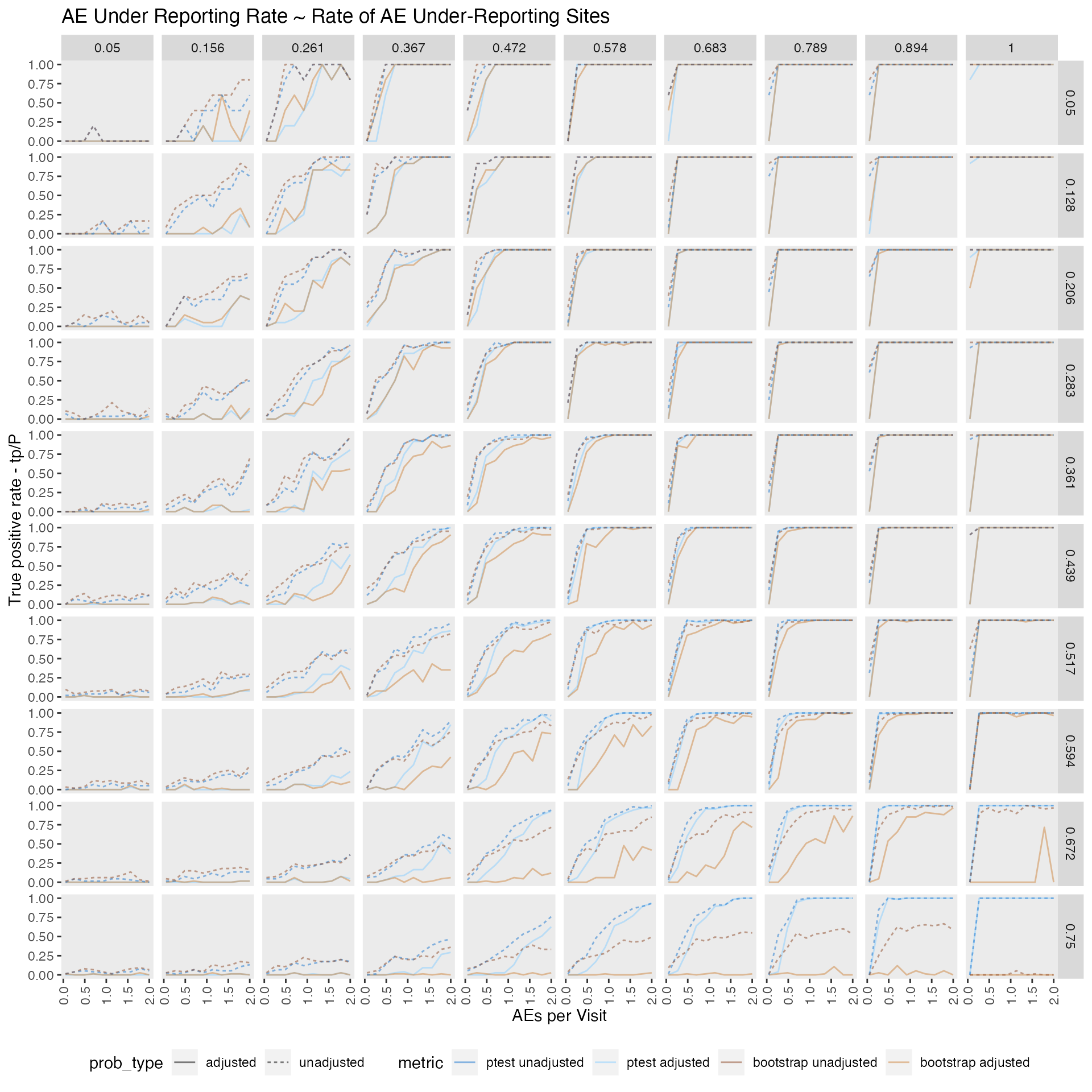
False positive rate FP/N
We can show that adjusting the AE under-reporting probability for the expected number of false positives is quite effective.As the false positive rate is almost zero for all tested scenarios. However, this also comes at a cost lowering the true positive rate as well.
p <- df_plot %>%
  mutate( fpr = fp/N) %>%
  select(ae_per_visit_mean, frac_site_with_ur, ur_rate, fpr, method, prob_type) %>%
  mutate_if(is.numeric, round, 3) %>%
  mutate(metric = case_when(method == "ptest" & prob_type == "unadjusted" ~ "ptest unadjusted",
                           method == "ptest" & prob_type == "adjusted" ~ "ptest adjusted",
                           method == "bootstrap" & prob_type == "unadjusted" ~ "bootstrap unadjusted",
                           method == "bootstrap" & prob_type == "adjusted" ~ "bootstrap adjusted"),
         metric = fct_relevel(metric, c("ptest unadjusted", "ptest adjusted",
                                        "bootstrap unadjusted", "bootstrap adjusted"))) %>%
  ggplot(aes(ae_per_visit_mean, fpr, color = metric, linetype = prob_type)) +
    geom_line(size = 0.5, alpha = 0.5) +
    facet_grid( frac_site_with_ur ~ ur_rate) +
    scale_color_manual(values = c("dodgerblue3", "skyblue1", "sienna4", "peru")) +
    theme(panel.grid = element_blank(), legend.position = "bottom",
          axis.text.x = element_text(angle = 90, vjust = 0.5)) +
    labs(title = "AE Under Reporting Rate by Rate of AE Under-Reporting Sites",
         y = "False positive rate - fp/N",
         x = "AEs per Visit")
p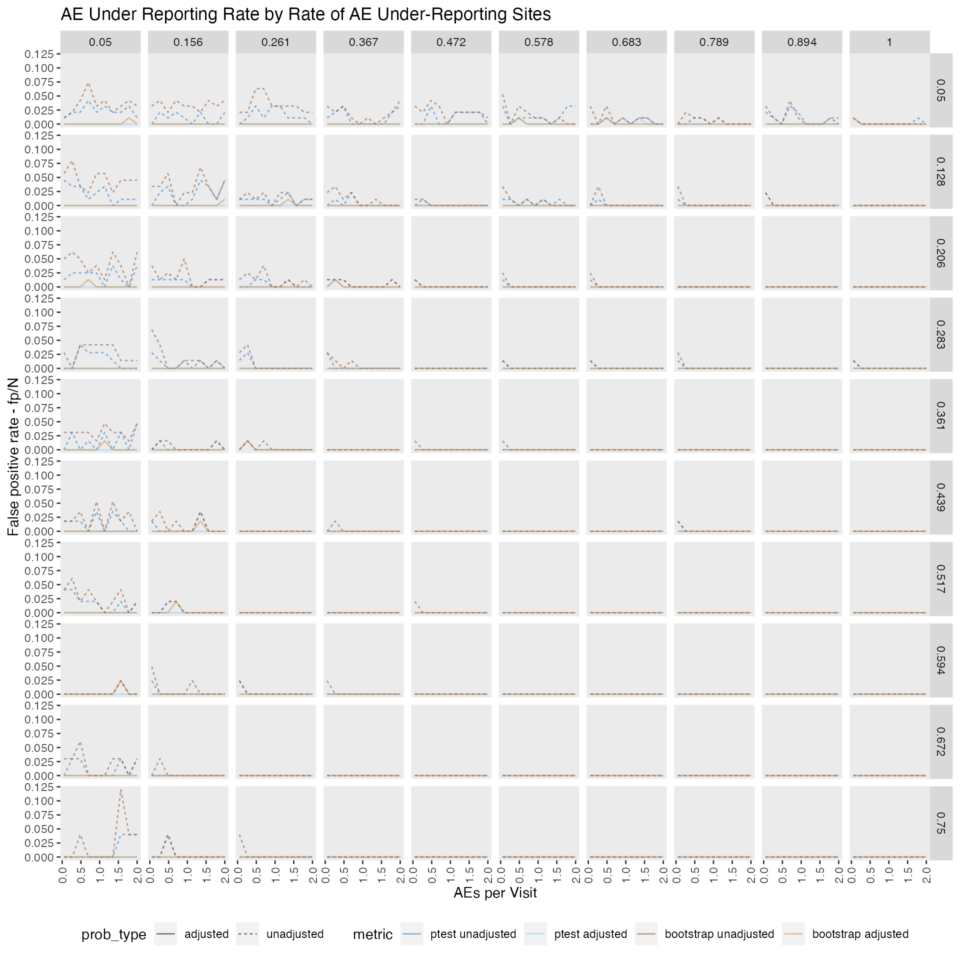
Conclusion
As already outlined in the introduction the true AE generating process is unlikely to be a standard poisson process. Therefore using a non-parametric test remains our recommended option unless that there is a reason to believe that 50% or more of all sites are under-reporting AEs. We also show that it is important to adjust for the expected false positive rate when calculating the final probabilities.
In general we can say that we do not recommend any method for detecting AE under-reporting that involves comparing AE counts if the ae per visit rate is 0.05 or lower.