BCVA data comparison between Bayesian and frequentist MMRMs
09/07/2024
Source:vignettes/bcva.Rmd
bcva.RmdAbout
This vignette uses the bcva_data dataset from the
mmrm package to compare a Bayesian MMRM fit, obtained by
brms.mmrm::brm_model(), and a frequentist MMRM fit,
obtained by mmrm::mmrm(). An overview of parameter
estimates and differences by type of MMRM is given in the summary (Tables 4 and 5) at the end.
Prerequisites
This comparison workflow requires the following packages.
> packages <- c(
+   "dplyr",
+   "tidyr",
+   "ggplot2",
+   "gt",
+   "gtsummary",
+   "purrr",
+   "parallel",
+   "brms.mmrm",
+   "mmrm",
+   "posterior"
+ )
> invisible(lapply(packages, library, character.only = TRUE))
We set a seed for the random number generator to ensure statistical reproducibility.
Data
Pre-processing
This analysis exercise uses the bcva_data dataset
contained in the mmrm package:
According to https://openpharma.github.io/mmrm/latest-tag/articles/mmrm_review_methods.html:
The BCVA dataset contains data from a randomized longitudinal ophthalmology trial evaluating the change in baseline corrected visual acuity (BCVA) over the course of 10 visits. BCVA corresponds to the number of letters read from a visual acuity chart.
The dataset is a tibble with 8605 rows and the following
notable variables.
-
USUBJID(subject ID) -
AVISIT(visit number, factor) -
VISITN(visit number, numeric) -
ARMCD(treatment,TRTorCTL) -
RACE(3-category race) -
BCVA_BL(BCVA at baseline) -
BCVA_CHG(BCVA change from baseline, primary endpoint for the analysis)
The rest of the pre-processing steps create factors for the study arm
and visit and apply the usual checking and standardization steps of
brms.mmrm::brm_data().
> bcva_data <- bcva_data |>
+   mutate(AVISIT = gsub("VIS0*", "VIS", as.character(AVISIT))) |>
+   brm_data(
+     outcome = "BCVA_CHG",
+     group = "ARMCD",
+     time = "AVISIT",
+     patient = "USUBJID",
+     baseline = "BCVA_BL",
+     reference_group = "CTL",
+     covariates = "RACE"
+   ) |>
+   brm_data_chronologize(order = "VISITN")
The following table shows the first rows of the dataset.
> head(bcva_data) |>
+   gt() |>
+ tab_caption(caption = md("Table 1. First rows of the pre-processed `bcva_data` dataset."))| USUBJID | AVISIT | VISITN | ARMCD | RACE | BCVA_BL | BCVA_CHG |
|---|---|---|---|---|---|---|
| 3 | VIS1 | 1 | CTL | Asian | 71.70881 | 5.058546 |
| 3 | VIS10 | 10 | CTL | Asian | 71.70881 | 10.152565 |
| 3 | VIS2 | 2 | CTL | Asian | 71.70881 | 4.018582 |
| 3 | VIS3 | 3 | CTL | Asian | 71.70881 | 3.572535 |
| 3 | VIS4 | 4 | CTL | Asian | 71.70881 | 4.822669 |
| 3 | VIS5 | 5 | CTL | Asian | 71.70881 | 7.348768 |
Descriptive statistics
Table of baseline characteristics:
> bcva_data |>
+   select(ARMCD, USUBJID, RACE, BCVA_BL) |>
+   distinct() |>
+   select(-USUBJID) |>
+   tbl_summary(
+     by = c(ARMCD),
+     statistic = list(
+       all_continuous() ~ "{mean} ({sd})",
+       all_categorical() ~ "{n} / {N} ({p}%)"
+     )
+   ) |>
+ modify_caption("Table 2. Baseline characteristics.")| Characteristic |
CTL N = 4941 |
TRT N = 5061 |
|---|---|---|
| RACE | ||
| Asian | 151 / 494 (31%) | 146 / 506 (29%) |
| Black | 149 / 494 (30%) | 168 / 506 (33%) |
| White | 194 / 494 (39%) | 192 / 506 (38%) |
| BCVA_BL | 75 (10) | 75 (10) |
| 1 n / N (%); Mean (SD) | ||
Table of change from baseline in BCVA over 52 weeks:
> bcva_data |>
+   pull(AVISIT) |>
+   unique() |>
+   sort() |>
+   purrr::map(
+     .f = ~ bcva_data |>
+       filter(AVISIT %in% .x) |>
+       tbl_summary(
+         by = ARMCD,
+         include = BCVA_CHG,
+         type = BCVA_CHG ~ "continuous2",
+         statistic = BCVA_CHG ~ c(
+           "{mean} ({sd})",
+           "{median} ({p25}, {p75})",
+           "{min}, {max}"
+         ),
+         label = list(BCVA_CHG = paste("Visit ", .x))
+       )
+   ) |>
+   tbl_stack(quiet = TRUE) |>
+ modify_caption("Table 3. Change from baseline.")| Characteristic |
CTL N = 494 |
TRT N = 506 |
|---|---|---|
| Visit VIS1 | ||
| Mean (SD) | 5.32 (1.23) | 5.86 (1.33) |
| Median (Q1, Q3) | 5.34 (4.51, 6.17) | 5.86 (4.98, 6.81) |
| Min, Max | 1.83, 9.02 | 2.28, 10.30 |
| Unknown | 12 | 5 |
| Visit VIS2 | ||
| Mean (SD) | 5.59 (1.49) | 6.33 (1.45) |
| Median (Q1, Q3) | 5.53 (4.64, 6.47) | 6.36 (5.34, 7.31) |
| Min, Max | 0.29, 10.15 | 2.35, 10.75 |
| Unknown | 13 | 7 |
| Visit VIS3 | ||
| Mean (SD) | 5.79 (1.61) | 6.79 (1.71) |
| Median (Q1, Q3) | 5.73 (4.64, 6.91) | 6.82 (5.66, 7.93) |
| Min, Max | 1.53, 11.46 | 1.13, 11.49 |
| Unknown | 23 | 17 |
| Visit VIS4 | ||
| Mean (SD) | 6.18 (1.73) | 7.29 (1.82) |
| Median (Q1, Q3) | 6.14 (5.05, 7.41) | 7.24 (6.05, 8.54) |
| Min, Max | 0.45, 11.49 | 2.07, 11.47 |
| Unknown | 36 | 18 |
| Visit VIS5 | ||
| Mean (SD) | 6.28 (1.97) | 7.68 (1.94) |
| Median (Q1, Q3) | 6.18 (4.96, 7.71) | 7.75 (6.48, 8.95) |
| Min, Max | 0.87, 11.53 | 2.24, 14.10 |
| Unknown | 40 | 35 |
| Visit VIS6 | ||
| Mean (SD) | 6.69 (1.97) | 8.31 (1.98) |
| Median (Q1, Q3) | 6.64 (5.26, 8.14) | 8.29 (6.92, 9.74) |
| Min, Max | 1.35, 12.95 | 1.93, 14.38 |
| Unknown | 84 | 48 |
| Visit VIS7 | ||
| Mean (SD) | 6.78 (2.09) | 8.78 (2.11) |
| Median (Q1, Q3) | 6.91 (5.46, 8.29) | 8.67 (7.44, 10.26) |
| Min, Max | -1.54, 11.99 | 3.21, 14.36 |
| Unknown | 106 | 78 |
| Visit VIS8 | ||
| Mean (SD) | 7.08 (2.25) | 9.40 (2.26) |
| Median (Q1, Q3) | 7.08 (5.55, 8.68) | 9.35 (7.96, 10.86) |
| Min, Max | 0.97, 13.71 | 2.28, 15.95 |
| Unknown | 123 | 86 |
| Visit VIS9 | ||
| Mean (SD) | 7.39 (2.33) | 10.01 (2.50) |
| Median (Q1, Q3) | 7.47 (5.76, 9.05) | 10.01 (8.19, 11.74) |
| Min, Max | 0.04, 14.61 | 4.22, 18.09 |
| Unknown | 167 | 114 |
| Visit VIS10 | ||
| Mean (SD) | 7.49 (2.58) | 10.59 (2.36) |
| Median (Q1, Q3) | 7.40 (5.73, 9.01) | 10.71 (9.03, 12.25) |
| Min, Max | -0.08, 15.75 | 3.24, 16.40 |
| Unknown | 213 | 170 |
The following figure shows the primary endpoint over the four study visits in the data.
> bcva_data |>
+   group_by(ARMCD) |>
+   ggplot(aes(x = AVISIT, y = BCVA_CHG, fill = factor(ARMCD))) +
+   geom_hline(yintercept = 0, col = "grey", linewidth = 1.2) +
+   geom_boxplot(na.rm = TRUE) +
+   labs(
+     x = "Visit",
+     y = "Change from baseline in BCVA",
+     fill = "Treatment"
+   ) +
+   scale_fill_manual(values = c("darkgoldenrod2", "coral2")) +
+   theme_bw()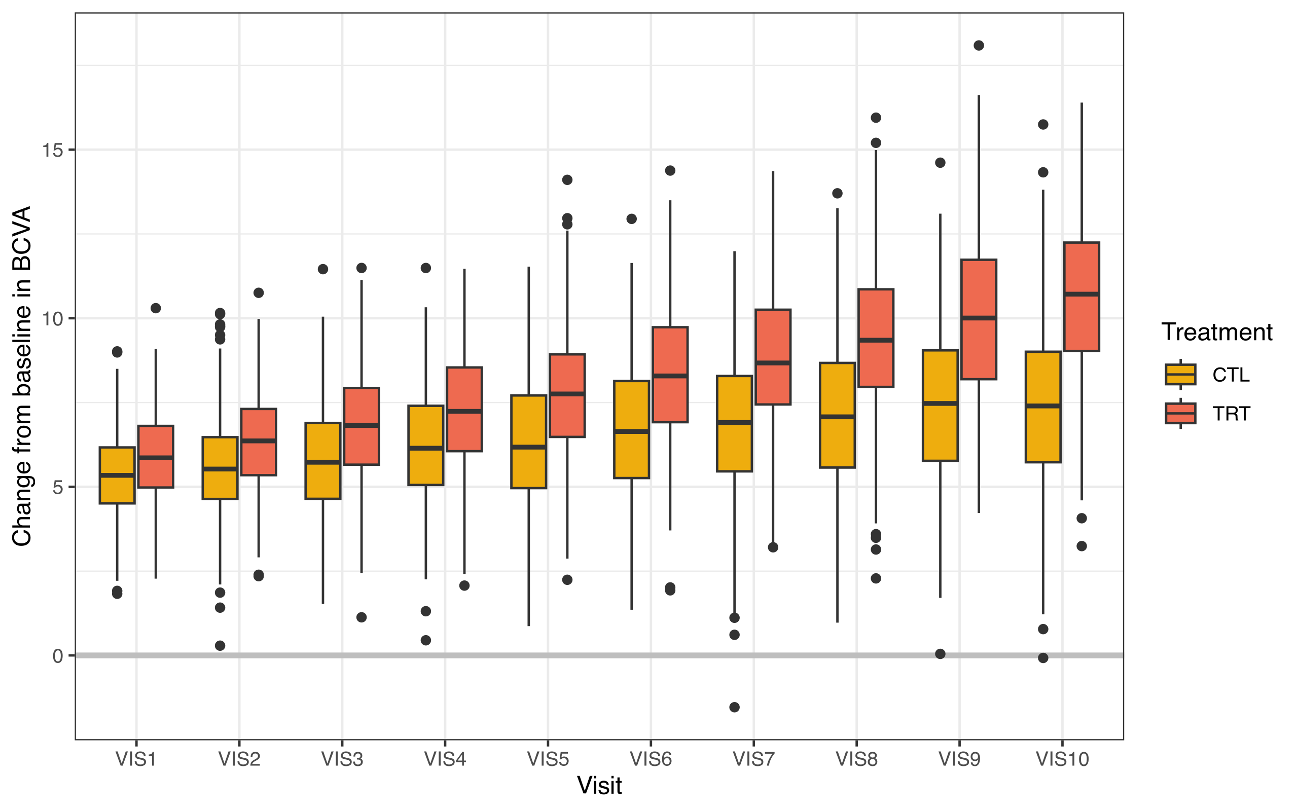
Figure 1. Change from baseline in BCVA over 4 visit time points.
Fitting MMRMs
Bayesian model
The formula for the Bayesian model includes additive effects for baseline, study visit, race, and study-arm-by-visit interaction.
> b_mmrm_formula <- brm_formula(
+   data = bcva_data,
+   intercept = TRUE,
+   baseline = TRUE,
+   group = FALSE,
+   time = TRUE,
+   baseline_time = FALSE,
+   group_time = TRUE,
+   correlation = "unstructured"
+ )
> print(b_mmrm_formula)
#> BCVA_CHG ~ BCVA_BL + ARMCD:AVISIT + AVISIT + RACE + unstr(time = AVISIT, gr = USUBJID)
#> sigma ~ 0 + AVISIT
We fit the model using brms.mmrm::brm_model(). The
computation takes several minutes because of the size of the dataset. To
ensure a good basis of comparison with the frequentist model, we put an
extremely diffuse prior on the intercept. The parameters already have
diffuse flexible priors by default.
> b_mmrm_fit <- brm_model(
+   data = filter(bcva_data, !is.na(BCVA_CHG)),
+   formula = b_mmrm_formula,
+   prior = brms::prior(class = "Intercept", prior = "student_t(3, 0, 1000)"),
+   iter = 10000,
+   warmup = 2000,
+   chains = 4,
+   cores = 4,
+   seed = 1,
+   refresh = 0
+ )
Here is a posterior summary of model parameters, including fixed effects and pairwise correlation among visits within patients.
> summary(b_mmrm_fit)
#>  Family: gaussian
#>   Links: mu = identity; sigma = log
#> Formula: BCVA_CHG ~ BCVA_BL + ARMCD:AVISIT + AVISIT + RACE + unstr(time = AVISIT, gr = USUBJID)
#>          sigma ~ 0 + AVISIT
#>    Data: data[!is.na(data[[attr(data, "brm_outcome")]]), ] (Number of observations: 8605)
#>   Draws: 4 chains, each with iter = 10000; warmup = 2000; thin = 1;
#>          total post-warmup draws = 32000
#>
#> Correlation Structures:
#>                     Estimate Est.Error l-95% CI u-95% CI Rhat Bulk_ESS Tail_ESS
#> cortime(VIS1,VIS2)      0.05      0.03    -0.01     0.11 1.00    63561    23159
#> cortime(VIS1,VIS3)      0.31      0.03     0.25     0.36 1.00    70330    25831
#> cortime(VIS2,VIS3)      0.05      0.03    -0.02     0.11 1.00    67715    22226
#> cortime(VIS1,VIS4)      0.21      0.03     0.15     0.27 1.00    46375    28108
#> cortime(VIS2,VIS4)      0.14      0.03     0.07     0.20 1.00    50232    27277
#> cortime(VIS3,VIS4)     -0.01      0.03    -0.07     0.05 1.00    50449    26940
#> cortime(VIS1,VIS5)      0.17      0.03     0.11     0.23 1.00    49366    27023
#> cortime(VIS2,VIS5)      0.12      0.03     0.05     0.18 1.00    53327    28297
#> cortime(VIS3,VIS5)     -0.01      0.03    -0.07     0.06 1.00    52752    26884
#> cortime(VIS4,VIS5)      0.38      0.03     0.32     0.43 1.00    49514    26959
#> cortime(VIS1,VIS6)      0.26      0.03     0.20     0.32 1.00    45483    26765
#> cortime(VIS2,VIS6)      0.20      0.03     0.14     0.27 1.00    48236    27168
#> cortime(VIS3,VIS6)      0.04      0.03    -0.02     0.11 1.00    51506    27189
#> cortime(VIS4,VIS6)      0.40      0.03     0.35     0.46 1.00    48730    25696
#> cortime(VIS5,VIS6)      0.39      0.03     0.34     0.45 1.00    55438    25998
#> cortime(VIS1,VIS7)      0.07      0.04    -0.00     0.13 1.00    66961    24586
#> cortime(VIS2,VIS7)      0.09      0.03     0.02     0.15 1.00    66564    23212
#> cortime(VIS3,VIS7)     -0.00      0.03    -0.07     0.07 1.00    62299    24284
#> cortime(VIS4,VIS7)      0.15      0.03     0.08     0.22 1.00    70101    23346
#> cortime(VIS5,VIS7)      0.19      0.03     0.13     0.26 1.00    71412    24243
#> cortime(VIS6,VIS7)      0.21      0.04     0.14     0.28 1.00    69307    23697
#> cortime(VIS1,VIS8)      0.05      0.04    -0.02     0.12 1.00    70424    22845
#> cortime(VIS2,VIS8)      0.10      0.04     0.03     0.17 1.00    71230    23497
#> cortime(VIS3,VIS8)     -0.03      0.04    -0.10     0.04 1.00    65689    22667
#> cortime(VIS4,VIS8)      0.17      0.03     0.10     0.24 1.00    68079    23681
#> cortime(VIS5,VIS8)      0.17      0.04     0.10     0.24 1.00    73436    24011
#> cortime(VIS6,VIS8)      0.16      0.04     0.09     0.23 1.00    68602    23567
#> cortime(VIS7,VIS8)      0.05      0.04    -0.02     0.13 1.00    68688    23661
#> cortime(VIS1,VIS9)      0.03      0.04    -0.04     0.10 1.00    70389    23613
#> cortime(VIS2,VIS9)     -0.01      0.04    -0.08     0.07 1.00    72988    22674
#> cortime(VIS3,VIS9)     -0.04      0.04    -0.12     0.03 1.00    73818    23450
#> cortime(VIS4,VIS9)      0.12      0.04     0.04     0.19 1.00    73299    24366
#> cortime(VIS5,VIS9)      0.09      0.04     0.02     0.16 1.00    72264    22069
#> cortime(VIS6,VIS9)      0.17      0.04     0.10     0.24 1.00    74018    24561
#> cortime(VIS7,VIS9)      0.02      0.04    -0.06     0.09 1.00    70521    22326
#> cortime(VIS8,VIS9)      0.06      0.04    -0.02     0.14 1.00    71301    22488
#> cortime(VIS1,VIS10)     0.02      0.04    -0.06     0.10 1.00    62930    25421
#> cortime(VIS2,VIS10)     0.13      0.04     0.05     0.20 1.00    58101    25684
#> cortime(VIS3,VIS10)     0.02      0.04    -0.06     0.10 1.00    60757    24802
#> cortime(VIS4,VIS10)     0.31      0.04     0.24     0.38 1.00    62762    26583
#> cortime(VIS5,VIS10)     0.24      0.04     0.16     0.31 1.00    66606    25076
#> cortime(VIS6,VIS10)     0.30      0.04     0.22     0.37 1.00    67998    23891
#> cortime(VIS7,VIS10)     0.06      0.04    -0.03     0.15 1.00    68944    23170
#> cortime(VIS8,VIS10)     0.09      0.04     0.01     0.18 1.00    71353    23530
#> cortime(VIS9,VIS10)     0.08      0.05    -0.01     0.17 1.00    65710    22799
#>
#> Regression Coefficients:
#>                      Estimate Est.Error l-95% CI u-95% CI Rhat Bulk_ESS
#> Intercept                4.29      0.17     3.96     4.62 1.00    56813
#> BCVA_BL                 -0.00      0.00    -0.01     0.00 1.00    59119
#> AVISIT2                  0.28      0.07     0.14     0.42 1.00    29890
#> AVISIT3                  0.46      0.07     0.33     0.59 1.00    44348
#> AVISIT4                  0.86      0.08     0.70     1.01 1.00    27610
#> AVISIT5                  0.96      0.09     0.79     1.13 1.00    29630
#> AVISIT6                  1.33      0.09     1.16     1.50 1.00    28672
#> AVISIT7                  1.42      0.11     1.21     1.63 1.00    34514
#> AVISIT8                  1.71      0.11     1.49     1.94 1.00    34167
#> AVISIT9                  2.00      0.13     1.75     2.25 1.00    35177
#> AVISIT10                 2.10      0.14     1.82     2.38 1.00    33084
#> RACEBlack                1.04      0.05     0.93     1.15 1.00    53517
#> RACEWhite                2.01      0.05     1.90     2.11 1.00    54553
#> AVISITVIS1:ARMCDTRT      0.54      0.06     0.41     0.66 1.00    34057
#> AVISITVIS2:ARMCDTRT      0.72      0.08     0.57     0.88 1.00    50542
#> AVISITVIS3:ARMCDTRT      1.01      0.09     0.83     1.19 1.00    48732
#> AVISITVIS4:ARMCDTRT      1.10      0.10     0.91     1.31 1.00    36650
#> AVISITVIS5:ARMCDTRT      1.38      0.12     1.16     1.61 1.00    38946
#> AVISITVIS6:ARMCDTRT      1.63      0.12     1.40     1.86 1.00    36052
#> AVISITVIS7:ARMCDTRT      2.02      0.14     1.74     2.29 1.00    45530
#> AVISITVIS8:ARMCDTRT      2.35      0.15     2.06     2.64 1.00    44496
#> AVISITVIS9:ARMCDTRT      2.66      0.16     2.33     2.98 1.00    44251
#> AVISITVIS10:ARMCDTRT     3.07      0.18     2.71     3.43 1.00    41207
#> sigma_AVISITVIS1        -0.01      0.02    -0.05     0.03 1.00    63843
#> sigma_AVISITVIS2         0.23      0.02     0.18     0.27 1.00    77180
#> sigma_AVISITVIS3         0.36      0.02     0.31     0.40 1.00    68147
#> sigma_AVISITVIS4         0.44      0.02     0.40     0.49 1.00    54719
#> sigma_AVISITVIS5         0.57      0.02     0.52     0.61 1.00    60122
#> sigma_AVISITVIS6         0.58      0.02     0.54     0.63 1.00    54741
#> sigma_AVISITVIS7         0.69      0.02     0.64     0.74 1.00    67848
#> sigma_AVISITVIS8         0.74      0.03     0.69     0.79 1.00    73959
#> sigma_AVISITVIS9         0.80      0.03     0.75     0.85 1.00    73387
#> sigma_AVISITVIS10        0.84      0.03     0.79     0.90 1.00    69664
#>                      Tail_ESS
#> Intercept               25046
#> BCVA_BL                 22844
#> AVISIT2                 25900
#> AVISIT3                 26347
#> AVISIT4                 26145
#> AVISIT5                 25959
#> AVISIT6                 25061
#> AVISIT7                 27504
#> AVISIT8                 26821
#> AVISIT9                 25947
#> AVISIT10                25296
#> RACEBlack               25805
#> RACEWhite               27113
#> AVISITVIS1:ARMCDTRT     27968
#> AVISITVIS2:ARMCDTRT     25650
#> AVISITVIS3:ARMCDTRT     27016
#> AVISITVIS4:ARMCDTRT     26502
#> AVISITVIS5:ARMCDTRT     25407
#> AVISITVIS6:ARMCDTRT     26418
#> AVISITVIS7:ARMCDTRT     26547
#> AVISITVIS8:ARMCDTRT     26731
#> AVISITVIS9:ARMCDTRT     26034
#> AVISITVIS10:ARMCDTRT    25859
#> sigma_AVISITVIS1        24881
#> sigma_AVISITVIS2        24252
#> sigma_AVISITVIS3        23768
#> sigma_AVISITVIS4        25358
#> sigma_AVISITVIS5        25761
#> sigma_AVISITVIS6        27071
#> sigma_AVISITVIS7        24330
#> sigma_AVISITVIS8        22567
#> sigma_AVISITVIS9        22205
#> sigma_AVISITVIS10       25249
#>
#> Draws were sampled using sampling(NUTS). For each parameter, Bulk_ESS
#> and Tail_ESS are effective sample size measures, and Rhat is the potential
#> scale reduction factor on split chains (at convergence, Rhat = 1).
Frequentist model
The formula for the frequentist model is the same, except for the different syntax for specifying the covariance structure of the MMRM. We fit the model below.
> f_mmrm_fit <- mmrm::mmrm(
+   formula = BCVA_CHG ~ BCVA_BL + ARMCD:AVISIT + AVISIT + RACE +
+     us(AVISIT | USUBJID),
+   data = mutate(
+     bcva_data,
+     AVISIT = factor(as.character(AVISIT), ordered = FALSE)
+   )
+ )
The parameter summaries of the frequentist model are below.
> summary(f_mmrm_fit)
#> mmrm fit
#>
#> Formula:     BCVA_CHG ~ BCVA_BL + ARMCD:AVISIT + AVISIT + RACE + us(AVISIT |
#>     USUBJID)
#> Data:
#> mutate(bcva_data, AVISIT = factor(as.character(AVISIT), ordered = FALSE)) (used
#> 8605 observations from 1000 subjects with maximum 10 timepoints)
#> Covariance:  unstructured (55 variance parameters)
#> Method:      Satterthwaite
#> Vcov Method: Asymptotic
#> Inference:   REML
#>
#> Model selection criteria:
#>      AIC      BIC   logLik deviance
#>  32181.0  32451.0 -16035.5  32071.0
#>
#> Coefficients:
#>                        Estimate Std. Error         df t value Pr(>|t|)
#> (Intercept)           4.288e+00  1.709e-01  1.065e+03  25.085  < 2e-16 ***
#> BCVA_BL              -9.935e-04  2.156e-03  9.905e+02  -0.461    0.645
#> AVISITVIS10           2.101e+00  1.400e-01  7.025e+02  15.003  < 2e-16 ***
#> AVISITVIS2            2.810e-01  7.067e-02  9.995e+02   3.976 7.51e-05 ***
#> AVISITVIS3            4.573e-01  6.716e-02  9.747e+02   6.809 1.71e-11 ***
#> AVISITVIS4            8.570e-01  7.636e-02  9.796e+02  11.222  < 2e-16 ***
#> AVISITVIS5            9.638e-01  8.634e-02  9.630e+02  11.163  < 2e-16 ***
#> AVISITVIS6            1.334e+00  8.650e-02  9.451e+02  15.421  < 2e-16 ***
#> AVISITVIS7            1.417e+00  1.071e-01  8.698e+02  13.233  < 2e-16 ***
#> AVISITVIS8            1.711e+00  1.145e-01  8.467e+02  14.944  < 2e-16 ***
#> AVISITVIS9            1.996e+00  1.283e-01  7.784e+02  15.549  < 2e-16 ***
#> RACEBlack             1.038e+00  5.496e-02  1.011e+03  18.891  < 2e-16 ***
#> RACEWhite             2.005e+00  5.198e-02  9.768e+02  38.573  < 2e-16 ***
#> AVISITVIS1:ARMCDTRT   5.391e-01  6.282e-02  9.859e+02   8.582  < 2e-16 ***
#> AVISITVIS10:ARMCDTRT  3.072e+00  1.815e-01  6.620e+02  16.929  < 2e-16 ***
#> AVISITVIS2:ARMCDTRT   7.248e-01  7.984e-02  9.803e+02   9.078  < 2e-16 ***
#> AVISITVIS3:ARMCDTRT   1.012e+00  9.163e-02  9.638e+02  11.039  < 2e-16 ***
#> AVISITVIS4:ARMCDTRT   1.104e+00  1.004e-01  9.653e+02  11.003  < 2e-16 ***
#> AVISITVIS5:ARMCDTRT   1.383e+00  1.147e-01  9.505e+02  12.065  < 2e-16 ***
#> AVISITVIS6:ARMCDTRT   1.630e+00  1.189e-01  9.157e+02  13.715  < 2e-16 ***
#> AVISITVIS7:ARMCDTRT   2.016e+00  1.382e-01  8.262e+02  14.592  < 2e-16 ***
#> AVISITVIS8:ARMCDTRT   2.347e+00  1.474e-01  8.041e+02  15.924  < 2e-16 ***
#> AVISITVIS9:ARMCDTRT   2.658e+00  1.644e-01  7.277e+02  16.172  < 2e-16 ***
#> ---
#> Signif. codes:  0 '***' 0.001 '**' 0.01 '*' 0.05 '.' 0.1 ' ' 1
#>
#> Covariance estimate:
#>         VIS1  VIS10    VIS2    VIS3    VIS4    VIS5   VIS6    VIS7    VIS8
#> VIS1  0.9713 0.0587  0.0630  0.4371  0.3315  0.3056 0.4688  0.1325  0.1020
#> VIS10 0.0587 5.3519  0.3761  0.0719  1.1478  0.9997 1.2558  0.3021  0.4658
#> VIS2  0.0630 0.3761  1.5618  0.0871  0.2684  0.2635 0.4636  0.2180  0.2776
#> VIS3  0.4371 0.0719  0.0871  2.0221 -0.0216 -0.0189 0.1102 -0.0048 -0.0993
#> VIS4  0.3315 1.1478  0.2684 -0.0216  2.4113  1.0475 1.1409  0.4625  0.5659
#> VIS5  0.3056 0.9997  0.2635 -0.0189  1.0475  3.0916 1.2593  0.6911  0.6308
#> VIS6  0.4688 1.2558  0.4636  0.1102  1.1409  1.2593 3.1853  0.7540  0.6094
#> VIS7  0.1325 0.3021  0.2180 -0.0048  0.4625  0.6911 0.7540  3.9272  0.2306
#> VIS8  0.1020 0.4658  0.2776 -0.0993  0.5659  0.6308 0.6094  0.2306  4.3272
#> VIS9  0.0611 0.4141 -0.0153 -0.1321  0.4085  0.3594 0.6823  0.0723  0.2683
#>          VIS9
#> VIS1   0.0611
#> VIS10  0.4141
#> VIS2  -0.0153
#> VIS3  -0.1321
#> VIS4   0.4085
#> VIS5   0.3594
#> VIS6   0.6823
#> VIS7   0.0723
#> VIS8   0.2683
#> VIS9   4.8635
Comparison
This section compares the Bayesian posterior parameter estimates from
brms.mmrm to the frequentist parameter estimates of the
mmrm package.
Extract estimates from Bayesian model
We extract and standardize the Bayesian estimates.
> b_mmrm_draws <- b_mmrm_fit |>
+   as_draws_df()
> visit_levels <- sort(unique(as.character(bcva_data$AVISIT)))
> for (level in visit_levels) {
+   name <- paste0("b_sigma_AVISIT", level)
+   b_mmrm_draws[[name]] <- exp(b_mmrm_draws[[name]])
+ }
> b_mmrm_summary <- b_mmrm_draws |>
+   summarize_draws() |>
+   select(variable, mean, sd) |>
+   filter(!(variable %in% c("Intercept", "lprior", "lp__"))) |>
+   rename(bayes_estimate = mean, bayes_se = sd) |>
+   mutate(
+     variable = variable |>
+       tolower() |>
+       gsub(pattern = "b_", replacement = "") |>
+       gsub(pattern = "b_sigma_AVISIT", replacement = "sigma_") |>
+       gsub(pattern = "cortime", replacement = "correlation") |>
+       gsub(pattern = "__", replacement = "_") |>
+       gsub(pattern = "avisitvis", replacement = "avisit")
+   )
Extract estimates from frequentist model
We extract and standardize the frequentist estimates.
> f_mmrm_fixed <- summary(f_mmrm_fit)$coefficients |>
+   as_tibble(rownames = "variable") |>
+   mutate(variable = tolower(variable)) |>
+   mutate(variable = gsub("(", "", variable, fixed = TRUE)) |>
+   mutate(variable = gsub(")", "", variable, fixed = TRUE)) |>
+   mutate(variable = gsub("avisitvis", "avisit", variable)) |>
+   rename(freq_estimate = Estimate, freq_se = `Std. Error`) |>
+   select(variable, freq_estimate, freq_se)
> f_mmrm_variance <- tibble(
+ variable = paste0("sigma_AVISIT", visit_levels) |>
+ tolower() |>
+ gsub(pattern = "avisitvis", replacement = "avisit"),
+ freq_estimate = sqrt(diag(f_mmrm_fit$cov))
+ )> f_diagonal_factor <- diag(1 / sqrt(diag(f_mmrm_fit$cov)))
> f_corr_matrix <- f_diagonal_factor %*% f_mmrm_fit$cov %*% f_diagonal_factor
> colnames(f_corr_matrix) <- visit_levels> f_mmrm_correlation <- f_corr_matrix |>
+ as.data.frame() |>
+ as_tibble() |>
+ mutate(x1 = visit_levels) |>
+ pivot_longer(
+ cols = -any_of("x1"),
+ names_to = "x2",
+ values_to = "freq_estimate"
+ ) |>
+ filter(
+ as.numeric(gsub("[^0-9]", "", x1)) < as.numeric(gsub("[^0-9]", "", x2))
+ ) |>
+ mutate(variable = sprintf("correlation_%s_%s", x1, x2)) |>
+ select(variable, freq_estimate)Summary
The first table below summarizes the parameter estimates from each model and the differences between estimates (Bayesian minus frequentist). The second table shows the standard errors of these estimates and differences between standard errors. In each table, the “Relative” column shows the relative difference (the difference divided by the frequentist quantity).
Because of the different statistical paradigms and estimation
procedures, especially regarding the covariance parameters, it would not
be realistic to expect the Bayesian and frequentist approaches to yield
virtually identical results. Nevertheless, the absolute and relative
differences in the table below show strong agreement between
brms.mmrm and mmrm.
> b_f_comparison <- full_join(
+   x = b_mmrm_summary,
+   y = f_mmrm_summary,
+   by = "variable"
+ ) |>
+   mutate(
+     diff_estimate = bayes_estimate - freq_estimate,
+     diff_relative_estimate = diff_estimate / freq_estimate,
+     diff_se = bayes_se - freq_se,
+     diff_relative_se = diff_se / freq_se
+   ) |>
+   select(variable, ends_with("estimate"), ends_with("se"))
> table_estimates <- b_f_comparison |>
+ select(variable, ends_with("estimate"))
> gt(table_estimates) |>
+ fmt_number(decimals = 4) |>
+ tab_caption(
+ caption = md(
+ paste(
+ "Table 4. Comparison of parameter estimates between",
+ "Bayesian and frequentist MMRMs."
+ )
+ )
+ ) |>
+ cols_label(
+ variable = "Variable",
+ bayes_estimate = "Bayesian",
+ freq_estimate = "Frequentist",
+ diff_estimate = "Difference",
+ diff_relative_estimate = "Relative"
+ )| Variable | Bayesian | Frequentist | Difference | Relative |
|---|---|---|---|---|
| intercept | 4.2889 | 4.2881 | 0.0009 | 0.0002 |
| bcva_bl | −0.0010 | −0.0010 | 0.0000 | 0.0143 |
| avisit2 | 0.2806 | 0.2810 | −0.0004 | −0.0014 |
| avisit3 | 0.4577 | 0.4573 | 0.0005 | 0.0010 |
| avisit4 | 0.8564 | 0.8570 | −0.0005 | −0.0006 |
| avisit5 | 0.9631 | 0.9638 | −0.0007 | −0.0007 |
| avisit6 | 1.3333 | 1.3339 | −0.0006 | −0.0005 |
| avisit7 | 1.4161 | 1.4167 | −0.0006 | −0.0005 |
| avisit8 | 1.7106 | 1.7107 | −0.0001 | −0.0001 |
| avisit9 | 1.9955 | 1.9956 | −0.0001 | 0.0000 |
| avisit10 | 2.0997 | 2.1005 | −0.0008 | −0.0004 |
| raceblack | 1.0385 | 1.0382 | 0.0002 | 0.0002 |
| racewhite | 2.0054 | 2.0051 | 0.0003 | 0.0002 |
| avisit1:armcdtrt | 0.5391 | 0.5391 | 0.0000 | −0.0001 |
| avisit2:armcdtrt | 0.7249 | 0.7248 | 0.0001 | 0.0001 |
| avisit3:armcdtrt | 1.0110 | 1.0115 | −0.0005 | −0.0005 |
| avisit4:armcdtrt | 1.1049 | 1.1042 | 0.0007 | 0.0007 |
| avisit5:armcdtrt | 1.3843 | 1.3834 | 0.0009 | 0.0007 |
| avisit6:armcdtrt | 1.6304 | 1.6301 | 0.0003 | 0.0002 |
| avisit7:armcdtrt | 2.0168 | 2.0160 | 0.0009 | 0.0004 |
| avisit8:armcdtrt | 2.3471 | 2.3469 | 0.0002 | 0.0001 |
| avisit9:armcdtrt | 2.6592 | 2.6585 | 0.0007 | 0.0003 |
| avisit10:armcdtrt | 3.0742 | 3.0723 | 0.0019 | 0.0006 |
| sigma_avisit1 | 0.9893 | 0.9855 | 0.0037 | 0.0038 |
| sigma_avisit2 | 1.2557 | 1.2497 | 0.0060 | 0.0048 |
| sigma_avisit3 | 1.4289 | 1.4220 | 0.0069 | 0.0048 |
| sigma_avisit4 | 1.5568 | 1.5528 | 0.0040 | 0.0026 |
| sigma_avisit5 | 1.7633 | 1.7583 | 0.0050 | 0.0028 |
| sigma_avisit6 | 1.7888 | 1.7847 | 0.0041 | 0.0023 |
| sigma_avisit7 | 1.9931 | 1.9817 | 0.0113 | 0.0057 |
| sigma_avisit8 | 2.0922 | 2.0802 | 0.0120 | 0.0058 |
| sigma_avisit9 | 2.2208 | 2.2053 | 0.0155 | 0.0070 |
| sigma_avisit10 | 2.3279 | 2.3134 | 0.0145 | 0.0063 |
| correlation_vis1_vis2 | 0.0489 | 0.0512 | −0.0023 | −0.0441 |
| correlation_vis1_vis3 | 0.3084 | 0.3119 | −0.0036 | −0.0114 |
| correlation_vis2_vis3 | 0.0482 | 0.0490 | −0.0008 | −0.0164 |
| correlation_vis1_vis4 | 0.2126 | 0.2166 | −0.0040 | −0.0184 |
| correlation_vis2_vis4 | 0.1351 | 0.1383 | −0.0033 | −0.0237 |
| correlation_vis3_vis4 | −0.0106 | −0.0098 | −0.0008 | 0.0869 |
| correlation_vis1_vis5 | 0.1722 | 0.1764 | −0.0041 | −0.0234 |
| correlation_vis2_vis5 | 0.1167 | 0.1199 | −0.0032 | −0.0265 |
| correlation_vis3_vis5 | −0.0082 | −0.0076 | −0.0006 | 0.0849 |
| correlation_vis4_vis5 | 0.3770 | 0.3836 | −0.0066 | −0.0173 |
| correlation_vis1_vis6 | 0.2617 | 0.2665 | −0.0048 | −0.0181 |
| correlation_vis2_vis6 | 0.2038 | 0.2079 | −0.0040 | −0.0194 |
| correlation_vis3_vis6 | 0.0422 | 0.0434 | −0.0012 | −0.0279 |
| correlation_vis4_vis6 | 0.4044 | 0.4117 | −0.0073 | −0.0177 |
| correlation_vis5_vis6 | 0.3941 | 0.4013 | −0.0072 | −0.0179 |
| correlation_vis1_vis7 | 0.0654 | 0.0679 | −0.0024 | −0.0360 |
| correlation_vis2_vis7 | 0.0857 | 0.0880 | −0.0023 | −0.0266 |
| correlation_vis3_vis7 | −0.0019 | −0.0017 | −0.0002 | 0.1039 |
| correlation_vis4_vis7 | 0.1464 | 0.1503 | −0.0040 | −0.0263 |
| correlation_vis5_vis7 | 0.1941 | 0.1983 | −0.0042 | −0.0214 |
| correlation_vis6_vis7 | 0.2083 | 0.2132 | −0.0048 | −0.0227 |
| correlation_vis1_vis8 | 0.0478 | 0.0497 | −0.0019 | −0.0382 |
| correlation_vis2_vis8 | 0.1044 | 0.1068 | −0.0024 | −0.0225 |
| correlation_vis3_vis8 | −0.0332 | −0.0336 | 0.0004 | −0.0112 |
| correlation_vis4_vis8 | 0.1712 | 0.1752 | −0.0040 | −0.0229 |
| correlation_vis5_vis8 | 0.1683 | 0.1725 | −0.0041 | −0.0240 |
| correlation_vis6_vis8 | 0.1597 | 0.1641 | −0.0045 | −0.0273 |
| correlation_vis7_vis8 | 0.0538 | 0.0559 | −0.0022 | −0.0392 |
| correlation_vis1_vis9 | 0.0269 | 0.0281 | −0.0012 | −0.0432 |
| correlation_vis2_vis9 | −0.0065 | −0.0056 | −0.0010 | 0.1708 |
| correlation_vis3_vis9 | −0.0416 | −0.0421 | 0.0005 | −0.0124 |
| correlation_vis4_vis9 | 0.1160 | 0.1193 | −0.0033 | −0.0273 |
| correlation_vis5_vis9 | 0.0898 | 0.0927 | −0.0029 | −0.0313 |
| correlation_vis6_vis9 | 0.1692 | 0.1733 | −0.0041 | −0.0238 |
| correlation_vis7_vis9 | 0.0153 | 0.0165 | −0.0013 | −0.0761 |
| correlation_vis8_vis9 | 0.0569 | 0.0585 | −0.0016 | −0.0267 |
| correlation_vis1_vis10 | 0.0229 | 0.0257 | −0.0029 | −0.1112 |
| correlation_vis2_vis10 | 0.1266 | 0.1301 | −0.0035 | −0.0267 |
| correlation_vis3_vis10 | 0.0217 | 0.0219 | −0.0002 | −0.0070 |
| correlation_vis4_vis10 | 0.3115 | 0.3195 | −0.0080 | −0.0251 |
| correlation_vis5_vis10 | 0.2385 | 0.2458 | −0.0073 | −0.0298 |
| correlation_vis6_vis10 | 0.2959 | 0.3041 | −0.0082 | −0.0271 |
| correlation_vis7_vis10 | 0.0631 | 0.0659 | −0.0028 | −0.0422 |
| correlation_vis8_vis10 | 0.0932 | 0.0968 | −0.0037 | −0.0377 |
| correlation_vis9_vis10 | 0.0781 | 0.0812 | −0.0031 | −0.0383 |
> table_se <- b_f_comparison |>
+   select(variable, ends_with("se")) |>
+   filter(!is.na(freq_se))
> gt(table_se) |>
+   fmt_number(decimals = 4) |>
+   tab_caption(
+     caption = md(
+       paste(
+         "Table 5. Comparison of parameter standard errors between",
+         "Bayesian and frequentist MMRMs."
+       )
+     )
+   ) |>
+   cols_label(
+     variable = "Variable",
+     bayes_se = "Bayesian",
+     freq_se = "Frequentist",
+     diff_se = "Difference",
+     diff_relative_se = "Relative"
+ )| Variable | Bayesian | Frequentist | Difference | Relative |
|---|---|---|---|---|
| intercept | 0.1695 | 0.1709 | −0.0015 | −0.0086 |
| bcva_bl | 0.0021 | 0.0022 | 0.0000 | −0.0100 |
| avisit2 | 0.0709 | 0.0707 | 0.0003 | 0.0038 |
| avisit3 | 0.0675 | 0.0672 | 0.0003 | 0.0052 |
| avisit4 | 0.0771 | 0.0764 | 0.0007 | 0.0094 |
| avisit5 | 0.0868 | 0.0863 | 0.0005 | 0.0055 |
| avisit6 | 0.0869 | 0.0865 | 0.0004 | 0.0042 |
| avisit7 | 0.1081 | 0.1071 | 0.0011 | 0.0102 |
| avisit8 | 0.1147 | 0.1145 | 0.0002 | 0.0017 |
| avisit9 | 0.1276 | 0.1283 | −0.0007 | −0.0057 |
| avisit10 | 0.1418 | 0.1400 | 0.0018 | 0.0130 |
| raceblack | 0.0548 | 0.0550 | −0.0001 | −0.0024 |
| racewhite | 0.0518 | 0.0520 | −0.0001 | −0.0029 |
| avisit1:armcdtrt | 0.0632 | 0.0628 | 0.0003 | 0.0054 |
| avisit2:armcdtrt | 0.0806 | 0.0798 | 0.0007 | 0.0093 |
| avisit3:armcdtrt | 0.0925 | 0.0916 | 0.0008 | 0.0092 |
| avisit4:armcdtrt | 0.1017 | 0.1004 | 0.0014 | 0.0136 |
| avisit5:armcdtrt | 0.1157 | 0.1147 | 0.0010 | 0.0088 |
| avisit6:armcdtrt | 0.1189 | 0.1189 | 0.0000 | 0.0003 |
| avisit7:armcdtrt | 0.1390 | 0.1382 | 0.0008 | 0.0060 |
| avisit8:armcdtrt | 0.1484 | 0.1474 | 0.0010 | 0.0066 |
| avisit9:armcdtrt | 0.1643 | 0.1644 | −0.0001 | −0.0004 |
| avisit10:armcdtrt | 0.1837 | 0.1815 | 0.0022 | 0.0122 |