FEV1 data comparison between Bayesian and frequentist MMRMs

About

This vignette provides an example comparison of a Bayesian MMRM fit, obtained by brms.mmrm::brm_model(), and a frequentist MMRM fit, obtained by mmrm::mmrm(). An overview of parameter estimates and differences by type of MMRM is given in the summary (Tables 4 and 5) at the end.

Prerequisites

This comparison workflow requires the following packages.

> packages <- c(
+   "dplyr",
+   "tidyr",
+   "ggplot2",
+   "gt",
+   "gtsummary",
+   "purrr",
+   "parallel",
+   "brms.mmrm",
+   "mmrm",
+   "emmeans",
+   "posterior"
+ )
> invisible(lapply(packages, library, character.only = TRUE))

We set a seed for the random number generator to ensure statistical reproducibility.

> set.seed(123L)

Data

Pre-processing

This analysis exercise uses the fev_dat dataset contained in the mmrm-package:

> data(fev_data, package = "mmrm")

It is an artificial (simulated) dataset of a clinical trial investigating the effect of an active treatment on FEV1 (forced expired volume in one second), compared to placebo. FEV1 is a measure of how quickly the lungs can be emptied and low levels may indicate chronic obstructive pulmonary disease (COPD).

The dataset is a tibble with 800 rows and 7 variables:

USUBJID (subject ID),
AVISIT (visit number),
ARMCD (treatment, TRT or PBO),
RACE (3-category race),
SEX (sex),
FEV1_BL (FEV1 at baseline, %),
FEV1 (FEV1 at study visits),
WEIGHT (weighting variable).

The primary endpoint for the analysis is change from baseline in FEV1, which we derive below and denote FEV1_CHG.

> fev_data <- fev_data |>
+   mutate("FEV1_CHG" = FEV1 - FEV1_BL)

The rest of the pre-processing steps create factors for the study arm and visit and apply the usual checking and standardization steps of brms.mmrm::brm_data().

> fev_data <- brm_data(
+   data = fev_data,
+   outcome = "FEV1_CHG",
+   role = "change",
+   group = "ARMCD",
+   time = "AVISIT",
+   patient = "USUBJID",
+   baseline = "FEV1_BL",
+   reference_group = "PBO",
+   covariates = c("RACE", "SEX")
+ ) |>
+   mutate(ARMCD = factor(ARMCD), AVISIT = factor(AVISIT))

The following table shows the first rows of the dataset.

> head(fev_data) |>
+   gt() |>
+   tab_caption(caption = md("Table 1. First rows of the pre-processed `fev_dat` dataset."))

Table 1. First rows of the pre-processed `fev_dat` dataset.
FEV1_CHG	FEV1_BL	ARMCD	AVISIT	USUBJID	RACE	SEX
NA	45.02477	PBO	VIS1	PT2	Asian	Male
-13.569552	45.02477	PBO	VIS2	PT2	Asian	Male
-8.145878	45.02477	PBO	VIS3	PT2	Asian	Male
3.783324	45.02477	PBO	VIS4	PT2	Asian	Male
NA	43.50070	PBO	VIS1	PT3	Black or African American	Female
-7.513705	43.50070	PBO	VIS2	PT3	Black or African American	Female

Descriptive statistics

Table of baseline characteristics:

> fev_data |>
+   select(ARMCD, USUBJID, SEX, RACE, FEV1_BL) |>
+   distinct() |>
+   select(-USUBJID) |>
+   tbl_summary(
+     by = c(ARMCD),
+     statistic = list(
+       all_continuous() ~ "{mean} ({sd})",
+       all_categorical() ~ "{n} / {N} ({p}%)"
+     )
+   ) |>
+   modify_caption("Table 2. Baseline characteristics.")

Table 2. Baseline characteristics.
Characteristic	PBO, N = 105¹	TRT, N = 95¹
SEX
Male	50 / 105 (48%)	44 / 95 (46%)
Female	55 / 105 (52%)	51 / 95 (54%)
RACE
Asian	38 / 105 (36%)	32 / 95 (34%)
Black or African American	46 / 105 (44%)	29 / 95 (31%)
White	21 / 105 (20%)	34 / 95 (36%)
FEV1_BL	40 (9)	40 (9)
¹ n / N (%); Mean (SD)

Table of change from baseline in FEV1 over 52 weeks:

> fev_data |>
+   pull(AVISIT) |>
+   unique() |>
+   sort() |>
+   purrr::map(
+     .f = ~ fev_data |>
+       filter(AVISIT %in% .x) |>
+       tbl_summary(
+         by = ARMCD,
+         include = FEV1_CHG,
+         type = FEV1_CHG ~ "continuous2",
+         statistic = FEV1_CHG ~ c(
+           "{mean} ({sd})",
+           "{median} ({p25}, {p75})",
+           "{min}, {max}"
+         ),
+         label = list(FEV1_CHG = paste("Visit ", .x))
+       )
+   ) |>
+   tbl_stack(quiet = TRUE) |>
+   modify_caption("Table 3. Change from baseline.")

Table 3. Change from baseline.
Characteristic	PBO, N = 105	TRT, N = 95
Visit VIS1
Mean (SD)	-8 (9)	-2 (10)
Median (IQR)	-9 (-16, 0)	-4 (-9, 7)
Range	-26, 12	-24, 20
Unknown	37	29
Visit VIS2
Mean (SD)	-3 (8)	2 (9)
Median (IQR)	-3 (-10, 1)	2 (-3, 8)
Range	-20, 15	-22, 23
Unknown	36	24
Visit VIS3
Mean (SD)	2 (8)	5 (9)
Median (IQR)	2 (-2, 8)	6 (0, 11)
Range	-15, 20	-19, 30
Unknown	34	37
Visit VIS4
Mean (SD)	8 (12)	13 (13)
Median (IQR)	6 (1, 18)	12 (5, 22)
Range	-20, 39	-14, 47
Unknown	38	28

The following figure shows the primary endpoint over the four study visits in the data.

> fev_data |>
+   group_by(ARMCD) |>
+   ggplot(aes(x = AVISIT, y = FEV1_CHG, fill = factor(ARMCD))) +
+   geom_hline(yintercept = 0, col = "grey", linewidth = 1.2) +
+   geom_boxplot(na.rm = TRUE) +
+   labs(
+     x = "Visit",
+     y = "Change from baseline in FEV1",
+     fill = "Treatment"
+   ) +
+   scale_fill_manual(values = c("darkgoldenrod2", "coral2")) +
+   theme_bw()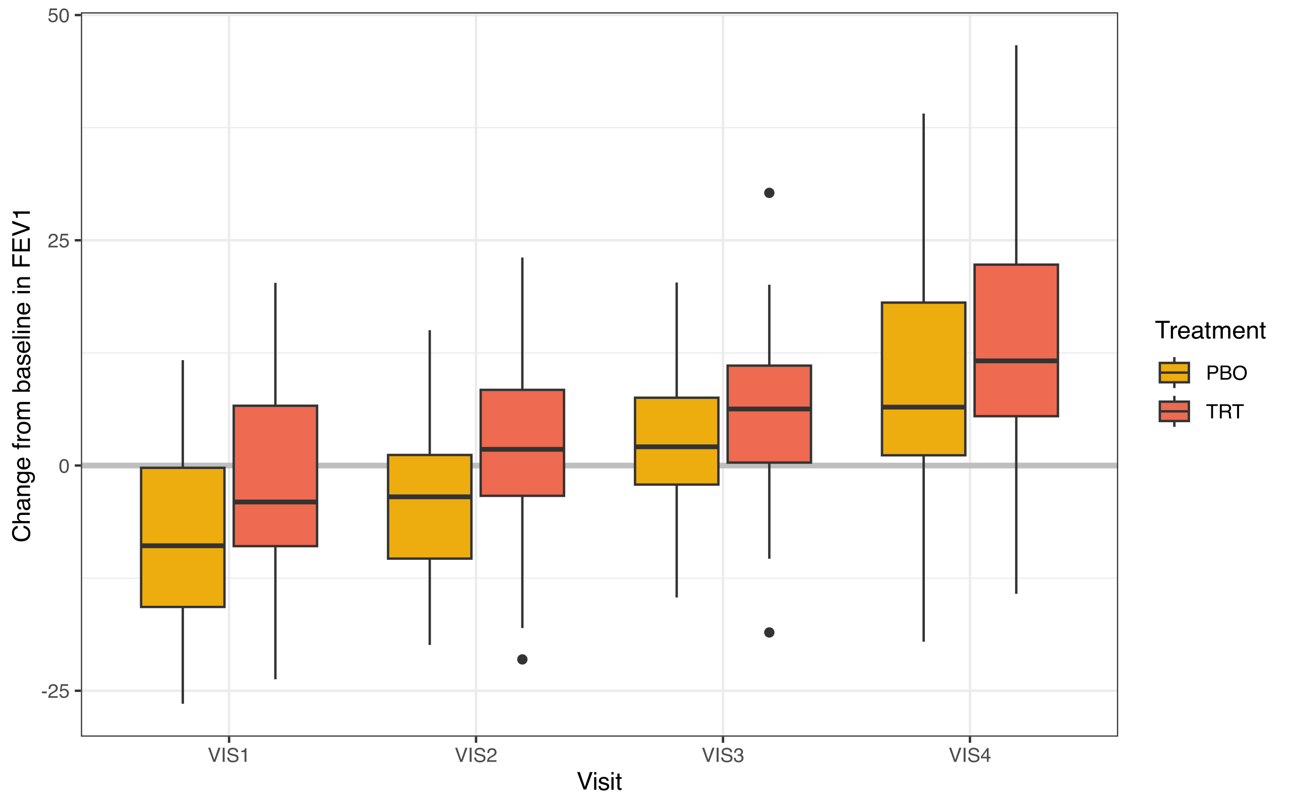

Figure 1. Change from baseline in FEV1 over 4 visit time points.

Fitting MMRMs

Bayesian model

The formula for the Bayesian model includes additive effects for baseline, study visit, race, sex, and study-arm-by-visit interaction.

> b_mmrm_formula <- brm_formula(
+   data = fev_data,
+   intercept = TRUE,
+   baseline = TRUE,
+   group = FALSE,
+   time = TRUE,
+   baseline_time = FALSE,
+   group_time = TRUE,
+   correlation = "unstructured"
+ )
> print(b_mmrm_formula)
#> FEV1_CHG ~ FEV1_BL + ARMCD:AVISIT + AVISIT + RACE + SEX + unstr(time = AVISIT, gr = USUBJID) 
#> sigma ~ 0 + AVISIT

We fit the model using brms.mmrm::brm_model(). To ensure a good basis of comparison with the frequentist model, we put an extremely diffuse prior on the intercept. The parameters already have diffuse flexible priors by default.

> b_mmrm_fit <- brm_model(
+   data = filter(fev_data, !is.na(FEV1_CHG)),
+   formula = b_mmrm_formula,
+   prior = brms::prior(class = "Intercept", prior = "student_t(3, 0, 1000)"),
+   iter = 10000,
+   warmup = 2000,
+   chains = 4,
+   cores = 1 + (detectCores() > 1),
+   refresh = 0
+ )

Here is a posterior summary of model parameters, including fixed effects and pairwise correlation among visits within patients.

> summary(b_mmrm_fit)
#>  Family: gaussian 
#>   Links: mu = identity; sigma = log 
#> Formula: FEV1_CHG ~ FEV1_BL + ARMCD:AVISIT + AVISIT + RACE + SEX + unstr(time = AVISIT, gr = USUBJID) 
#>          sigma ~ 0 + AVISIT
#>    Data: data[!is.na(data[[attr(data, "brm_outcome")]]), ] (Number of observations: 537) 
#>   Draws: 4 chains, each with iter = 10000; warmup = 2000; thin = 1;
#>          total post-warmup draws = 32000
#> 
#> Correlation Structures:
#>                    Estimate Est.Error l-95% CI u-95% CI Rhat Bulk_ESS Tail_ESS
#> cortime(VIS1,VIS2)     0.36      0.08     0.18     0.52 1.00    57792    24956
#> cortime(VIS1,VIS3)     0.14      0.10    -0.06     0.33 1.00    56286    23466
#> cortime(VIS2,VIS3)     0.04      0.10    -0.16     0.23 1.00    59573    24133
#> cortime(VIS1,VIS4)     0.17      0.11    -0.06     0.38 1.00    55344    23991
#> cortime(VIS2,VIS4)     0.11      0.09    -0.06     0.28 1.00    56072    24575
#> cortime(VIS3,VIS4)     0.01      0.10    -0.19     0.21 1.00    55495    24208
#> 
#> Population-Level Effects: 
#>                            Estimate Est.Error l-95% CI u-95% CI Rhat Bulk_ESS Tail_ESS
#> Intercept                     24.35      1.41    21.57    27.12 1.00    51092    26082
#> FEV1_BL                       -0.84      0.03    -0.90    -0.79 1.00    65718    24255
#> AVISITVIS2                     4.80      0.82     3.20     6.41 1.00    34670    26507
#> AVISITVIS3                    10.38      0.83     8.76    12.00 1.00    32763    25123
#> AVISITVIS4                    15.19      1.34    12.52    17.84 1.00    38951    25700
#> RACEBlackorAfricanAmerican     1.41      0.58     0.27     2.56 1.00    52375    25352
#> RACEWhite                      5.45      0.62     4.23     6.67 1.00    50708    26395
#> SEXFemale                      0.34      0.51    -0.66     1.34 1.00    56857    23425
#> AVISITVIS1:ARMCDTRT            3.99      1.07     1.89     6.09 1.00    34463    26924
#> AVISITVIS2:ARMCDTRT            3.93      0.83     2.30     5.55 1.00    53992    22708
#> AVISITVIS3:ARMCDTRT            2.98      0.67     1.66     4.29 1.00    55787    23907
#> AVISITVIS4:ARMCDTRT            4.40      1.70     1.05     7.75 1.00    50570    24724
#> sigma_AVISITVIS1               1.83      0.06     1.71     1.95 1.00    55678    23281
#> sigma_AVISITVIS2               1.59      0.06     1.47     1.71 1.00    54337    25242
#> sigma_AVISITVIS3               1.33      0.06     1.20     1.45 1.00    57630    24234
#> sigma_AVISITVIS4               2.28      0.06     2.16     2.41 1.00    58888    23768
#> 
#> Draws were sampled using sampling(NUTS). For each parameter, Bulk_ESS
#> and Tail_ESS are effective sample size measures, and Rhat is the potential
#> scale reduction factor on split chains (at convergence, Rhat = 1).

Frequentist model

The formula for the frequentist model is the same, except for the different syntax for specifying the covariance structure of the MMRM. We fit the model below.

> f_mmrm_fit <- mmrm::mmrm(
+   formula = FEV1_CHG ~ FEV1_BL + ARMCD:AVISIT + AVISIT + RACE + SEX +
+     us(AVISIT | USUBJID),
+   data = fev_data
+ )

The parameter summaries of the frequentist model are below.

> summary(f_mmrm_fit)
#> mmrm fit
#> 
#> Formula:     FEV1_CHG ~ FEV1_BL + ARMCD:AVISIT + AVISIT + RACE + SEX + us(AVISIT |  
#>     USUBJID)
#> Data:        fev_data (used 537 observations from 197 subjects with maximum 4 
#> timepoints)
#> Covariance:  unstructured (10 variance parameters)
#> Method:      Satterthwaite
#> Vcov Method: Asymptotic
#> Inference:   REML
#> 
#> Model selection criteria:
#>      AIC      BIC   logLik deviance 
#>   3381.4   3414.2  -1680.7   3361.4 
#> 
#> Coefficients: 
#>                                Estimate Std. Error        df t value Pr(>|t|)    
#> (Intercept)                    24.35372    1.40754 257.97000  17.302  < 2e-16 ***
#> FEV1_BL                        -0.84022    0.02777 190.27000 -30.251  < 2e-16 ***
#> AVISITVIS2                      4.79036    0.79848 144.82000   5.999 1.51e-08 ***
#> AVISITVIS3                     10.36601    0.81318 157.08000  12.748  < 2e-16 ***
#> AVISITVIS4                     15.19231    1.30857 139.25000  11.610  < 2e-16 ***
#> RACEBlack or African American   1.41921    0.57874 169.56000   2.452 0.015211 *  
#> RACEWhite                       5.45679    0.61626 157.54000   8.855 1.65e-15 ***
#> SEXFemale                       0.33812    0.49273 166.43000   0.686 0.493529    
#> AVISITVIS1:ARMCDTRT             3.98329    1.04540 142.32000   3.810 0.000206 ***
#> AVISITVIS2:ARMCDTRT             3.93076    0.81351 142.26000   4.832 3.46e-06 ***
#> AVISITVIS3:ARMCDTRT             2.98372    0.66567 129.61000   4.482 1.61e-05 ***
#> AVISITVIS4:ARMCDTRT             4.40400    1.66049 132.88000   2.652 0.008970 ** 
#> ---
#> Signif. codes:  0 '***' 0.001 '**' 0.01 '*' 0.05 '.' 0.1 ' ' 1
#> 
#> Covariance estimate:
#>         VIS1    VIS2    VIS3    VIS4
#> VIS1 37.8301 11.3255  3.4796 10.6844
#> VIS2 11.3255 23.5476  0.7760  5.5103
#> VIS3  3.4796  0.7760 13.8037  0.5683
#> VIS4 10.6844  5.5103  0.5683 92.9625

Comparison

This section compares the Bayesian posterior parameter estimates from brms.mmrm to the frequentist parameter estimates of the mmrm package.

Extract estimates from Bayesian model

We extract and standardize the Bayesian estimates.

> b_mmrm_draws <- b_mmrm_fit |>
+   as_draws_df()
> visit_levels <- sort(unique(as.character(fev_data$AVISIT)))
> for (level in visit_levels) {
+   name <- paste0("b_sigma_AVISIT", level)
+   b_mmrm_draws[[name]] <- exp(b_mmrm_draws[[name]])
+ }
> b_mmrm_summary <- b_mmrm_draws |>
+   summarize_draws() |>
+   select(variable, mean, sd) |>
+   filter(!(variable %in% c("lprior", "lp__"))) |>
+   rename(bayes_estimate = mean, bayes_se = sd) |>
+   mutate(
+     variable = variable |>
+       tolower() |>
+       gsub(pattern = "b_", replacement = "") |>
+       gsub(pattern = "b_sigma_AVISIT", replacement = "sigma_") |>
+       gsub(pattern = "cortime", replacement = "correlation") |>
+       gsub(pattern = "__", replacement = "_")
+   )

Extract estimates from frequentist model

We extract and standardize the frequentist estimates.

> f_mmrm_fixed <- summary(f_mmrm_fit)$coefficients |>
+   as_tibble(rownames = "variable") |>
+   mutate(variable = tolower(variable)) |>
+   mutate(variable = gsub("(", "", variable, fixed = TRUE)) |>
+   mutate(variable = gsub(")", "", variable, fixed = TRUE)) |>
+   rename(freq_estimate = Estimate, freq_se = `Std. Error`) |>
+   select(variable, freq_estimate, freq_se)

> f_mmrm_variance <- tibble(
+   variable = paste0("sigma_AVISIT", visit_levels) |> tolower(),
+   freq_estimate = sqrt(diag(f_mmrm_fit$cov))
+ )

> f_diagonal_factor <- diag(1 / sqrt(diag(f_mmrm_fit$cov)))
> f_corr_matrix <- f_diagonal_factor %*% f_mmrm_fit$cov %*% f_diagonal_factor
> colnames(f_corr_matrix) <- visit_levels

> f_mmrm_correlation <- f_corr_matrix |>
+   as.data.frame() |>
+   as_tibble() |>
+   mutate(x1 = visit_levels) |>
+   pivot_longer(
+     cols = -any_of("x1"),
+     names_to = "x2",
+     values_to = "freq_estimate"
+   ) |>
+   filter(
+     as.numeric(gsub("[^0-9]", "", x1)) < as.numeric(gsub("[^0-9]", "", x2))
+   ) |>
+   mutate(variable = sprintf("correlation_%s_%s", x1, x2)) |>
+   select(variable, freq_estimate)

> f_mmrm_summary <- bind_rows(
+   f_mmrm_fixed,
+   f_mmrm_variance,
+   f_mmrm_correlation
+ ) |>
+   mutate(variable = gsub("\\s+", "", variable) |> tolower())

Summary

The first table below summarizes the parameter estimates from each model and the differences between estimates (Bayesian minus frequentist). The second table shows the standard errors of these estimates and differences between standard errors. In each table, the “Relative” column shows the relative difference (the difference divided by the frequentist quantity).

Because of the different statistical paradigms and estimation procedures, especially regarding the covariance parameters, it would not be realistic to expect the Bayesian and frequentist approaches to yield virtually identical results. Nevertheless, the absolute and relative differences in the table below show strong agreement between brms.mmrm and mmrm.

> b_f_comparison <- full_join(
+   x = b_mmrm_summary,
+   y = f_mmrm_summary,
+   by = "variable"
+ ) |>
+   mutate(
+     diff_estimate = bayes_estimate - freq_estimate,
+     diff_relative_estimate = diff_estimate / freq_estimate,
+     diff_se = bayes_se - freq_se,
+     diff_relative_se = diff_se / freq_se
+   ) |>
+   select(variable, ends_with("estimate"), ends_with("se"))

> table_estimates <- b_f_comparison |>
+   select(variable, ends_with("estimate"))
> gt(table_estimates) |>
+   fmt_number(decimals = 4) |>
+   tab_caption(
+     caption = md(
+       paste(
+         "Table 4. Comparison of parameter estimates between",
+         "Bayesian and frequentist MMRMs."
+       )
+     )
+   ) |>
+   cols_label(
+     variable = "Variable",
+     bayes_estimate = "Bayesian",
+     freq_estimate = "Frequentist",
+     diff_estimate = "Difference",
+     diff_relative_estimate = "Relative"
+   )

Table 4. Comparison of parameter estimates between Bayesian and frequentist MMRMs.
Variable	Bayesian	Frequentist	Difference	Relative
intercept	24.3483	24.3537	−0.0054	−0.0002
fev1_bl	−0.8402	−0.8402	0.0000	0.0000
avisitvis2	4.7983	4.7904	0.0079	0.0017
avisitvis3	10.3790	10.3660	0.0130	0.0012
avisitvis4	15.1918	15.1923	−0.0005	0.0000
raceblackorafricanamerican	1.4128	1.4192	−0.0064	−0.0045
racewhite	5.4493	5.4568	−0.0075	−0.0014
sexfemale	0.3446	0.3381	0.0064	0.0191
avisitvis1:armcdtrt	3.9909	3.9833	0.0076	0.0019
avisitvis2:armcdtrt	3.9329	3.9308	0.0022	0.0006
avisitvis3:armcdtrt	2.9784	2.9837	−0.0054	−0.0018
avisitvis4:armcdtrt	4.4001	4.4040	−0.0039	−0.0009
sigma_avisitvis1	6.2313	6.1506	0.0807	0.0131
sigma_avisitvis2	4.9149	4.8526	0.0623	0.0128
sigma_avisitvis3	3.7761	3.7153	0.0607	0.0163
sigma_avisitvis4	9.8009	9.6417	0.1592	0.0165
correlation_vis1_vis2	0.3604	0.3795	−0.0191	−0.0503
correlation_vis1_vis3	0.1414	0.1523	−0.0109	−0.0717
correlation_vis2_vis3	0.0397	0.0430	−0.0034	−0.0786
correlation_vis1_vis4	0.1672	0.1802	−0.0129	−0.0717
correlation_vis2_vis4	0.1102	0.1178	−0.0076	−0.0646
correlation_vis3_vis4	0.0135	0.0159	−0.0024	−0.1483

> table_se <- b_f_comparison |>
+   select(variable, ends_with("se")) |>
+   filter(!is.na(freq_se))
> gt(table_se) |>
+   fmt_number(decimals = 4) |>
+   tab_caption(
+     caption = md(
+       paste(
+         "Table 5. Comparison of parameter standard errors between",
+         "Bayesian and frequentist MMRMs."
+       )
+     )
+   ) |>
+   cols_label(
+     variable = "Variable",
+     bayes_se = "Bayesian",
+     freq_se = "Frequentist",
+     diff_se = "Difference",
+     diff_relative_se = "Relative"
+   )

Table 5. Comparison of parameter standard errors between Bayesian and frequentist MMRMs.
Variable	Bayesian	Frequentist	Difference	Relative
intercept	1.4117	1.4075	0.0042	0.0030
fev1_bl	0.0277	0.0278	−0.0001	−0.0020
avisitvis2	0.8240	0.7985	0.0256	0.0320
avisitvis3	0.8319	0.8132	0.0188	0.0231
avisitvis4	1.3444	1.3086	0.0358	0.0273
raceblackorafricanamerican	0.5832	0.5787	0.0044	0.0076
racewhite	0.6221	0.6163	0.0058	0.0095
sexfemale	0.5083	0.4927	0.0156	0.0317
avisitvis1:armcdtrt	1.0722	1.0454	0.0268	0.0256
avisitvis2:armcdtrt	0.8255	0.8135	0.0120	0.0147
avisitvis3:armcdtrt	0.6725	0.6657	0.0069	0.0103
avisitvis4:armcdtrt	1.7016	1.6605	0.0411	0.0248

27/03/2024