Statistical Performance • simaerep

Load

suppressPackageStartupMessages(library(dplyr))
suppressPackageStartupMessages(library(tibble))
suppressPackageStartupMessages(library(tidyr))
suppressPackageStartupMessages(library(simaerep))
suppressPackageStartupMessages(library(purrr))
suppressPackageStartupMessages(library(furrr))
suppressPackageStartupMessages(library(stringr))
suppressPackageStartupMessages(library(patchwork))

Introduction

{simaerep} calculates site-specific event reporting probabilities based on bootstrap simulations that replace individual patients with other patients from the same study that have at least the same number of visits. This makes it ideal for monitoring event reporting of ongoing trials in which not all sites and patients are starting in the trial at the same time and in which the event rates are not constant over the entire treatment cycle.

The statistical performance of {simaerep} is thus best measured against a data set that includes ongoing studies in different stages and non-constant event rates. For this we use a snapshot of our portfolio data to simulate a test data set from which we subsequently remove or add a specific percentage of events to create over- and under-reporting scenarios. We will then measure statistical performance of {simaerep} and compare it to those of other statistical methods.

We have previously evaluated {simaerep} for detecting adverse events under-reporting in a joint industry publication using a similar approach.

Koneswarakantha, B., Adyanthaya, R., Emerson, J. et al. An Open-Source R Package for Detection of Adverse Events Under-Reporting in Clinical Trials: Implementation and Validation by the IMPALA (Inter coMPany quALity Analytics) Consortium. Ther Innov Regul Sci 58, 591–599 (2024). https://doi.org/10.1007/s43441-024-00631-8

Test Data

Portfolio Configuration and Event Rates

The portfolio configuration will be used to generate compliant test data that is similar to a realistic portfolio of studies in which all sites are compliant. We will subsequently remove a percentage of AEs from each study site and calculate AE under-reporting statistics to calculate overall detection thresholds. The portfolio configuration should give a minimal description of the portfolio without violating data privacy laws or competitive intellectual property. We propose to include the following metrics into the portfolio configuration:

site parameters:

mean of all maximum patient visits
sd of of all maximum patient visits
total number patients

study parameters:

mean AE per visit

The information contained in a portfolio configuration is very scarce and thus can be shared more easily within the industry. We can use those parameters to simulate test data for assessing {simaerep} performance on a given portfolio.

We start with our standard input data set df_visit from which we extract the portfolio configuration and the event rates using simaerep::get_portf_config and simaerep::get_portf_event_rates:

This workflow will automatically:

remove patients with 0 visits
minimum number of patients per study
minimum number of sites per study
anonymize study and site IDs

df_visit1 <- sim_test_data_study(
  n_pat = 100,
  n_sites = 10,
  ratio_out = 0.4,
  factor_event_rate = - 0.6,
  event_rates = c(0.3, 1, 0.7, 0.1),
  study_id = "A"
)

df_visit2 <- sim_test_data_study(
  n_pat = 100,
  n_sites = 10,
  ratio_out = 0.2,
  factor_event_rate = - 0.1,
  event_rates = c(1, 0.5, 0.3, 0.3),
  study_id = "B"
)

df_visit <- bind_rows(df_visit1, df_visit2)


df_config <- simaerep::get_portf_config(
  df_visit,
  anonymize = TRUE,
  min_pat_per_study = 100,
  min_sites_per_study = 10
)

df_config %>%
  head(25) %>%
  knitr::kable()

study_id	event_per_visit_mean	site_id	max_visit_sd	max_visit_mean	n_pat
0001	0.1517349	0001	4.175324	19.1	10
0001	0.1517349	0002	5.108816	18.1	10
0001	0.1517349	0003	3.011091	18.8	10
0001	0.1517349	0004	3.366502	18.0	10
0001	0.1517349	0005	3.831159	18.7	10
0001	0.1517349	0006	2.708013	19.0	10
0001	0.1517349	0007	1.885618	20.0	10
0001	0.1517349	0008	3.333333	20.0	10
0001	0.1517349	0009	3.765339	22.2	10
0001	0.1517349	0010	2.898275	19.2	10
0002	0.3070175	0001	4.237400	17.8	10
0002	0.3070175	0002	3.622461	19.3	10
0002	0.3070175	0003	3.272783	18.6	10
0002	0.3070175	0004	4.648775	20.5	10
0002	0.3070175	0005	3.368152	20.3	10
0002	0.3070175	0006	4.083844	20.3	10
0002	0.3070175	0007	4.900113	19.3	10
0002	0.3070175	0008	3.622461	20.3	10
0002	0.3070175	0009	3.604010	17.9	10
0002	0.3070175	0010	3.308239	19.5	10

df_event_rates <- simaerep::get_portf_event_rates(df_visit)

df_event_rates %>%
  filter(dense_rank(study_id) == 1) %>%
  knitr::kable()

study_id	visit	event_rate	n_pat
0001	1	0.0000000	100
0001	2	0.8400000	100
0001	3	0.6100000	100
0001	4	0.1000000	100
0001	5	0.0700000	100
0001	6	0.0606061	99
0001	7	0.0707071	99
0001	8	0.0606061	99
0001	9	0.0909091	99
0001	10	0.0909091	99
0001	11	0.1111111	99
0001	12	0.0909091	99
0001	13	0.0927835	97
0001	14	0.0729167	96
0001	15	0.0659341	91
0001	16	0.0114943	87
0001	17	0.1250000	80
0001	18	0.0694444	72
0001	19	0.0476190	63
0001	20	0.1224490	49
0001	21	0.0500000	40
0001	22	0.0384615	26
0001	23	0.0666667	15
0001	24	0.0000000	12
0001	25	0.2857143	7
0001	26	0.0000000	3

The configuration and the event rates can be used to simulate a new set of portfolio data with simaerep::sim_test_data_portfolio

simaerep::sim_test_data_portfolio(df_config, df_event_rates, progress = TRUE)

## # A tibble: 3,751 × 8
##    study_id event_per_visit_mean site_id max_visit_sd max_visit_mean patient_id
##    <chr>                   <dbl> <chr>          <dbl>          <dbl> <chr>     
##  1 0001                    0.152 0001            4.18           19.1 0001      
##  2 0001                    0.152 0001            4.18           19.1 0001      
##  3 0001                    0.152 0001            4.18           19.1 0001      
##  4 0001                    0.152 0001            4.18           19.1 0001      
##  5 0001                    0.152 0001            4.18           19.1 0001      
##  6 0001                    0.152 0001            4.18           19.1 0001      
##  7 0001                    0.152 0001            4.18           19.1 0001      
##  8 0001                    0.152 0001            4.18           19.1 0001      
##  9 0001                    0.152 0001            4.18           19.1 0001      
## 10 0001                    0.152 0001            4.18           19.1 0001      
## # ℹ 3,741 more rows
## # ℹ 2 more variables: visit <int>, n_event <dbl>

Load Portfolio

To simulate a realistic test set with ongoing studies we load snapshots from our portfolio. We can use future package to set the number of workers for parallel processing.

df_config <- readr::read_csv("ae_conf_20240220.csv") %>%
  rename_with(~stringr::str_replace(., "ae_", "event_")) %>%
  rename(site_id = site_number)

df_event_rates <- readr::read_csv("ae_rates_20240220.csv") %>%
  rename_with(~stringr::str_replace(., "ae_", "event_")) %>%
  rename(visit = cum_visit)


suppressPackageStartupMessages(library(furrr))

plan(multisession, workers = 6)

df_portf <- sim_test_data_portfolio(
  df_config,
  df_event_rates,
  progress = TRUE,
  parallel = TRUE
)

plan(sequential)

Simulating Reporting Outlier

Next we will write a function that uses simaerep and other statistical methods to detect reporting outlier. We will apply the following.

remove or add events directly from the data set and not from an aggregated metric using simaerep::sim_out()
set threshold for confusion matrix so that all methods have similar fpr
test the following {simaerep} parameters:
- classic algorithm
- inframe algorithm with visit_med75
- inframe algorithm
- inframe algorithm w/o multiplicity correction
test the following outlier detection methods
- box-plot
- funnel-plot Zink et al. 2018

Functions

funnel <- function(df) {
  
  df %>%
    filter(visit == max(visit), .by = "patient_id") %>%
    summarise(
      Metric = sum(.data$n_event) / sum(.data$visit),
      n_event = sum(n_event),
      visit = sum(visit),
      .by = "site_id"
    ) %>%
    mutate(
          vMu = sum(.data$n_event) / sum(.data$visit),
          z_0 = ifelse(.data$vMu == 0,
            0,
            (.data$Metric - .data$vMu) /
              sqrt(.data$vMu / .data$visit)
          ),
          phi = mean(.data$z_0^2),
          z_i = ifelse(.data$vMu == 0 | .data$phi == 0,
            0,
            (.data$Metric - .data$vMu) /
              sqrt(.data$phi * .data$vMu / .data$visit)
          )
    )
}

box <- function(df) {

  df <- df %>%
    filter(visit == max(visit), .by = "patient_id") %>%
    summarise(
      event_per_visit = sum(.data$n_event) / sum(.data$visit),
      .by = "site_id"
    )
  
  bx <- boxplot.stats(df$event_per_visit)

  df <- df %>%
    mutate(
      box_out = event_per_visit < bx$stats[1] | event_per_visit > bx$stats[5]
    )
  
}


perf <- function(df_visit, study_id, site_id, factor_event) {

  df_vs_study <- df_visit %>%
    simaerep::sim_out(study_id, site_id, factor_event)
  
  remove(df_visit)
  
  df_classic <- df_vs_study %>%
    simaerep(inframe = FALSE, progress = FALSE, check = FALSE) %>%
    .$df_eval %>%
    filter(.data$site_id == .env$site_id)

  df_inframe <- df_vs_study %>%
    simaerep(check = FALSE, progress = FALSE) %>%
    .$df_eval %>%
    filter(.data$site_id == .env$site_id)
  
  df_inframe_visit_med75 <- df_vs_study %>%
    simaerep(visit_med75 = TRUE, check = FALSE, progress = FALSE) %>%
    .$df_eval %>%
    filter(.data$site_id == .env$site_id)

  funnel_zi <- funnel(df_vs_study) %>%
    filter(.data$site_id == .env$site_id) %>%
    pull(z_i)
  
  box_out <- box(df_vs_study) %>%
    filter(.data$site_id == .env$site_id) %>%
    pull(box_out)
  
  df <- tibble(
    score_classic = df_classic$prob,
    score_classic_no_mult = df_classic$prob_no_mult,
    score_inframe = df_inframe$event_prob,
    score_inframe_no_mult = df_inframe$event_prob_no_mult,
    score_inframe_visit_med75 = df_inframe_visit_med75$event_prob,
    score_inframe_visit_med75_no_mult = df_inframe_visit_med75$event_prob_no_mult,
    score_funnel_zi = funnel_zi,
    score_box_out = as.integer(box_out),
    stat_classic_visit_med75 = df_classic$visit_med75,
    stat_classic_n_pat_with_med75 = df_classic$n_pat_with_med75,
    stat_classic_mean_event_site_med75 = df_classic$mean_event_site_med75,
    stat_classic_mean_event_study_med75 = df_classic$mean_event_study_med75,
    stat_inframe_visit_med75 = df_inframe_visit_med75$visit_med75,
    stat_inframe_visit_med75_n_pat_with_med75 = df_inframe_visit_med75$n_pat_with_med75,
    stat_inframe_visit_med75_events_per_visit_site = df_inframe_visit_med75$event_per_visit_site,
    stat_inframe_visit_med75_events_per_visit_study = df_inframe_visit_med75$event_per_visit_site,
    stat_inframe_n_pat = df_inframe$n_pat,
    stat_inframe_events_per_visit_site = df_inframe$event_per_visit_site,
    stat_inframe_events_per_visit_study = df_inframe$event_per_visit_study,
  )
  
  if (! any(str_detect(colnames(df), "no_mult"))) {
    stop("no scores w/o multiplicity correction available")
  }
    
  return(df)
}

# 50% over-reporting
perf(df_portf, study_id = "0010", site_id = "15153", factor_event = 0.5) %>% unlist()

##                                   score_classic 
##                                       0.8045000 
##                           score_classic_no_mult 
##                                       0.9970000 
##                                   score_inframe 
##                                       0.8289375 
##                           score_inframe_no_mult 
##                                       0.9860000 
##                       score_inframe_visit_med75 
##                                       0.8390000 
##               score_inframe_visit_med75_no_mult 
##                                       0.9940000 
##                                 score_funnel_zi 
##                                       2.1931127 
##                                   score_box_out 
##                                       0.0000000 
##                    stat_classic_visit_med75.80% 
##                                       7.0000000 
##                   stat_classic_n_pat_with_med75 
##                                       5.0000000 
##              stat_classic_mean_event_site_med75 
##                                       3.9000000 
##             stat_classic_mean_event_study_med75 
##                                       2.0576324 
##                    stat_inframe_visit_med75.80% 
##                                       7.0000000 
##       stat_inframe_visit_med75_n_pat_with_med75 
##                                       5.0000000 
##  stat_inframe_visit_med75_events_per_visit_site 
##                                       0.5571429 
## stat_inframe_visit_med75_events_per_visit_study 
##                                       0.5571429 
##                              stat_inframe_n_pat 
##                                       9.0000000 
##              stat_inframe_events_per_visit_site 
##                                       0.4615385 
##             stat_inframe_events_per_visit_study 
##                                       0.2937692

# 50% under-reporting
perf(df_portf, study_id = "0010", site_id = "15153", factor_event = - 0.5) %>% unlist()

##                                   score_classic 
##                                     -0.03400000 
##                           score_classic_no_mult 
##                                     -0.99400000 
##                                   score_inframe 
##                                     -0.27550000 
##                           score_inframe_no_mult 
##                                     -0.98000000 
##                       score_inframe_visit_med75 
##                                     -0.83900000 
##               score_inframe_visit_med75_no_mult 
##                                     -0.99900000 
##                                 score_funnel_zi 
##                                     -2.24765772 
##                                   score_box_out 
##                                      0.00000000 
##                    stat_classic_visit_med75.80% 
##                                      7.00000000 
##                   stat_classic_n_pat_with_med75 
##                                      5.00000000 
##              stat_classic_mean_event_site_med75 
##                                      0.50000000 
##             stat_classic_mean_event_study_med75 
##                                      2.05763240 
##                    stat_inframe_visit_med75.80% 
##                                      7.00000000 
##       stat_inframe_visit_med75_n_pat_with_med75 
##                                      5.00000000 
##  stat_inframe_visit_med75_events_per_visit_site 
##                                      0.07142857 
## stat_inframe_visit_med75_events_per_visit_study 
##                                      0.07142857 
##                              stat_inframe_n_pat 
##                                      9.00000000 
##              stat_inframe_events_per_visit_site 
##                                      0.15384615 
##             stat_inframe_events_per_visit_study 
##                                      0.29052308

Grid

df_grid <- df_portf %>%
  distinct(study_id, site_id) %>%
  # to reduce calculation time we only take every xth study
  filter(dense_rank(study_id)%%5 == 0) %>%
  mutate(factor_event = list(c( -1, -.75, -.5, -.25, -.1, 0, 0.1, 0.25, 0.5, 0.75, 1))) %>%
  unnest(factor_event)

df_grid

## # A tibble: 49,720 × 3
##    study_id site_id factor_event
##    <chr>    <chr>          <dbl>
##  1 0005     4480           -1   
##  2 0005     4480           -0.75
##  3 0005     4480           -0.5 
##  4 0005     4480           -0.25
##  5 0005     4480           -0.1 
##  6 0005     4480            0   
##  7 0005     4480            0.1 
##  8 0005     4480            0.25
##  9 0005     4480            0.5 
## 10 0005     4480            0.75
## # ℹ 49,710 more rows

Apply

Again we use the furrr and the future package for parallel processing. simaerep::purrr_bar is a wrapper around furrr functions that enables the progressr package to display a progress bar.

plan(multisession, workers = 6)

progressr::with_progress(
  df_perf <- df_grid %>%
    mutate(
      perf = simaerep::purrr_bar(
        list(study_id, site_id, factor_event),
        .purrr = furrr::future_pmap,
        .f = function(x, y, z) perf(df_portf, x, y, z),
        .purrr_args = list(.options = furrr_options(seed = TRUE)),
        .steps = nrow(.)
      )
    )
)

plan(sequential)


df_perf %>%
  unnest(perf) %>%
  readr::write_csv("perf.csv")

df_perf <- readr::read_csv("perf.csv", show_col_types = FALSE)

df_perf_long <- df_perf %>%
  pivot_longer(cols = - c(study_id, site_id, factor_event), names_to = "type", values_to = "score") %>%
  filter(startsWith(type, "score_")) %>%
  mutate(
    type = stringr::str_replace(type, "score_", ""),
    # we use the same cut-off for over- and under-reporting
    score = abs(score)
  )

Evaluation

Thresholds

We set the thresholds so that we get a fpr of 0.01.

Note that this results in probability thresholds ~ 0.99 for scores w/o multiplicity correction and in the recommended funnel plot score threshold of -2.

target_fpr <- 0.01

df_thresh <- df_perf_long %>%
  group_by(type) %>%
  nest() %>%
  ungroup() %>%
  mutate(
    data = map(data, ~ filter(., factor_event == 0)),
    thresh = map_dbl(data, ~ quantile(pull(., score), 1 - target_fpr)),
  ) %>%
  select(type, thresh)
  
df_thresh

## # A tibble: 8 × 2
##   type                        thresh
##   <chr>                        <dbl>
## 1 classic                      0.849
## 2 classic_no_mult              0.995
## 3 inframe                      0.849
## 4 inframe_no_mult              0.996
## 5 inframe_visit_med75          0.848
## 6 inframe_visit_med75_no_mult  0.996
## 7 funnel_zi                    2.70 
## 8 box_out                      1

Aggregate

get_prop_test_ci95 <- function(..., ix) {
  
  stopifnot(ix %in% c(1, 2))
  
  tryCatch(
    prop.test(...)$conf.int[ix],
    error = function(cnd) c(NA, NA)[ix]
  )
}

df_aggr <- df_perf_long %>%
  left_join(df_thresh, by = "type") %>%
  mutate(
    is_out = score >= thresh,
    is_out = ifelse(type == "box_out", score == 1, is_out)
  ) %>%
  summarise(
    n = n(),
    .by = c(type, factor_event, is_out)
  ) %>%
  pivot_wider(
    names_from = is_out,
    values_from = n,
    names_prefix = "is_out_",
    values_fill = 0
  ) %>%
  mutate(
    n_sites = is_out_TRUE + is_out_FALSE,
    ratio = is_out_TRUE / n_sites,
    ratio_type = ifelse(factor_event == 0, "fpr", "tpr"),
    ci95_low = map2_dbl(is_out_TRUE, n_sites, ~ get_prop_test_ci95(.x, .y, ix = 1)),
    ci95_high = map2_dbl(is_out_TRUE, n_sites, ~ get_prop_test_ci95(.x, .y, ix = 2)),
    type_strip = str_replace(type, "_no_mult", ""),
    has_mult = ! str_detect(type, "no_mult") & ! type %in% c("funnel_zi", "box_out")
  )

Table

Methods:

classic: classic algorithm
inframe: new algorithm using table operations
inframe w/o multiplicity correction: new algorithm using table operations without multiplicity corrections
inframe visit_med75: new algorithm using table operations and visit_med75
funnel_zi: funnel plot derived outlier detection
box_out: box plot derived outlier detection

FN: false negatives TP: true positives

df_aggr %>%
  select(method = type_strip, has_mult, factor_event, FN = is_out_FALSE, TP = is_out_TRUE, n_sites, ratio_type, ratio, ci95_low, ci95_high) %>%
  knitr::kable(digits = 4)

method	has_mult	factor_event	FN	TP	n_sites	ratio_type	ratio	ci95_low	ci95_high
classic	TRUE	-1.00	1432	3088	4520	tpr	0.6832	0.6694	0.6967
classic	FALSE	-1.00	958	3562	4520	tpr	0.7881	0.7758	0.7998
inframe	TRUE	-1.00	1384	3136	4520	tpr	0.6938	0.6801	0.7072
inframe	FALSE	-1.00	1054	3466	4520	tpr	0.7668	0.7542	0.7790
inframe_visit_med75	TRUE	-1.00	1556	2964	4520	tpr	0.6558	0.6417	0.6696
inframe_visit_med75	FALSE	-1.00	1155	3365	4520	tpr	0.7445	0.7314	0.7571
funnel_zi	FALSE	-1.00	1643	2877	4520	tpr	0.6365	0.6223	0.6505
box_out	FALSE	-1.00	776	3744	4520	tpr	0.8283	0.8169	0.8391
classic	TRUE	-0.75	1772	2748	4520	tpr	0.6080	0.5935	0.6222
classic	FALSE	-0.75	1295	3225	4520	tpr	0.7135	0.7000	0.7266
inframe	TRUE	-0.75	1789	2731	4520	tpr	0.6042	0.5898	0.6185
inframe	FALSE	-0.75	1441	3079	4520	tpr	0.6812	0.6673	0.6947
inframe_visit_med75	TRUE	-0.75	1832	2688	4520	tpr	0.5947	0.5802	0.6090
inframe_visit_med75	FALSE	-0.75	1460	3060	4520	tpr	0.6770	0.6631	0.6906
funnel_zi	FALSE	-0.75	2423	2097	4520	tpr	0.4639	0.4493	0.4786
box_out	FALSE	-0.75	2337	2183	4520	tpr	0.4830	0.4683	0.4977
classic	TRUE	-0.50	2634	1886	4520	tpr	0.4173	0.4028	0.4318
classic	FALSE	-0.50	2250	2270	4520	tpr	0.5022	0.4875	0.5169
inframe	TRUE	-0.50	2718	1802	4520	tpr	0.3987	0.3844	0.4131
inframe	FALSE	-0.50	2395	2125	4520	tpr	0.4701	0.4555	0.4848
inframe_visit_med75	TRUE	-0.50	2637	1883	4520	tpr	0.4166	0.4022	0.4311
inframe_visit_med75	FALSE	-0.50	2335	2185	4520	tpr	0.4834	0.4687	0.4981
funnel_zi	FALSE	-0.50	3411	1109	4520	tpr	0.2454	0.2329	0.2582
box_out	FALSE	-0.50	3636	884	4520	tpr	0.1956	0.1842	0.2075
classic	TRUE	-0.25	3883	637	4520	tpr	0.1409	0.1310	0.1515
classic	FALSE	-0.25	3579	941	4520	tpr	0.2082	0.1965	0.2204
inframe	TRUE	-0.25	3917	603	4520	tpr	0.1334	0.1237	0.1437
inframe	FALSE	-0.25	3665	855	4520	tpr	0.1892	0.1779	0.2010
inframe_visit_med75	TRUE	-0.25	3886	634	4520	tpr	0.1403	0.1303	0.1508
inframe_visit_med75	FALSE	-0.25	3656	864	4520	tpr	0.1912	0.1798	0.2030
funnel_zi	FALSE	-0.25	4309	211	4520	tpr	0.0467	0.0408	0.0533
box_out	FALSE	-0.25	4307	213	4520	tpr	0.0471	0.0412	0.0538
classic	TRUE	-0.10	4444	76	4520	tpr	0.0168	0.0134	0.0211
classic	FALSE	-0.10	4367	153	4520	tpr	0.0338	0.0289	0.0396
inframe	TRUE	-0.10	4436	84	4520	tpr	0.0186	0.0149	0.0231
inframe	FALSE	-0.10	4393	127	4520	tpr	0.0281	0.0236	0.0334
inframe_visit_med75	TRUE	-0.10	4454	66	4520	tpr	0.0146	0.0114	0.0187
inframe_visit_med75	FALSE	-0.10	4402	118	4520	tpr	0.0261	0.0217	0.0313
funnel_zi	FALSE	-0.10	4469	51	4520	tpr	0.0113	0.0085	0.0149
box_out	FALSE	-0.10	4323	197	4520	tpr	0.0436	0.0379	0.0501
classic	TRUE	0.00	4474	46	4520	fpr	0.0102	0.0075	0.0137
classic	FALSE	0.00	4474	46	4520	fpr	0.0102	0.0075	0.0137
inframe	TRUE	0.00	4473	47	4520	fpr	0.0104	0.0077	0.0139
inframe	FALSE	0.00	4472	48	4520	fpr	0.0106	0.0079	0.0142
inframe_visit_med75	TRUE	0.00	4474	46	4520	fpr	0.0102	0.0075	0.0137
inframe_visit_med75	FALSE	0.00	4472	48	4520	fpr	0.0106	0.0079	0.0142
funnel_zi	FALSE	0.00	4474	46	4520	fpr	0.0102	0.0075	0.0137
box_out	FALSE	0.00	4253	267	4520	fpr	0.0591	0.0525	0.0664
classic	TRUE	0.10	4399	121	4520	tpr	0.0268	0.0223	0.0320
classic	FALSE	0.10	4318	202	4520	tpr	0.0447	0.0389	0.0512
inframe	TRUE	0.10	4392	128	4520	tpr	0.0283	0.0238	0.0337
inframe	FALSE	0.10	4330	190	4520	tpr	0.0420	0.0365	0.0484
inframe_visit_med75	TRUE	0.10	4389	131	4520	tpr	0.0290	0.0244	0.0344
inframe_visit_med75	FALSE	0.10	4342	178	4520	tpr	0.0394	0.0340	0.0456
funnel_zi	FALSE	0.10	4401	119	4520	tpr	0.0263	0.0219	0.0315
box_out	FALSE	0.10	4161	359	4520	tpr	0.0794	0.0718	0.0878
classic	TRUE	0.25	3855	665	4520	tpr	0.1471	0.1370	0.1579
classic	FALSE	0.25	3551	969	4520	tpr	0.2144	0.2026	0.2267
inframe	TRUE	0.25	3870	650	4520	tpr	0.1438	0.1338	0.1545
inframe	FALSE	0.25	3654	866	4520	tpr	0.1916	0.1803	0.2034
inframe_visit_med75	TRUE	0.25	3844	676	4520	tpr	0.1496	0.1394	0.1604
inframe_visit_med75	FALSE	0.25	3591	929	4520	tpr	0.2055	0.1939	0.2177
funnel_zi	FALSE	0.25	4031	489	4520	tpr	0.1082	0.0994	0.1177
box_out	FALSE	0.25	3855	665	4520	tpr	0.1471	0.1370	0.1579
classic	TRUE	0.50	2662	1858	4520	tpr	0.4111	0.3967	0.4256
classic	FALSE	0.50	2327	2193	4520	tpr	0.4852	0.4705	0.4999
inframe	TRUE	0.50	2722	1798	4520	tpr	0.3978	0.3835	0.4122
inframe	FALSE	0.50	2463	2057	4520	tpr	0.4551	0.4405	0.4697
inframe_visit_med75	TRUE	0.50	2677	1843	4520	tpr	0.4077	0.3934	0.4223
inframe_visit_med75	FALSE	0.50	2370	2150	4520	tpr	0.4757	0.4610	0.4903
funnel_zi	FALSE	0.50	3020	1500	4520	tpr	0.3319	0.3182	0.3458
box_out	FALSE	0.50	3021	1499	4520	tpr	0.3316	0.3180	0.3456
classic	TRUE	0.75	1920	2600	4520	tpr	0.5752	0.5606	0.5897
classic	FALSE	0.75	1623	2897	4520	tpr	0.6409	0.6267	0.6549
inframe	TRUE	0.75	1978	2542	4520	tpr	0.5624	0.5478	0.5769
inframe	FALSE	0.75	1757	2763	4520	tpr	0.6113	0.5969	0.6255
inframe_visit_med75	TRUE	0.75	1915	2605	4520	tpr	0.5763	0.5618	0.5908
inframe_visit_med75	FALSE	0.75	1682	2838	4520	tpr	0.6279	0.6136	0.6420
funnel_zi	FALSE	0.75	2106	2414	4520	tpr	0.5341	0.5194	0.5487
box_out	FALSE	0.75	2136	2384	4520	tpr	0.5274	0.5128	0.5421
classic	TRUE	1.00	1394	3126	4520	tpr	0.6916	0.6779	0.7050
classic	FALSE	1.00	1146	3374	4520	tpr	0.7465	0.7335	0.7590
inframe	TRUE	1.00	1461	3059	4520	tpr	0.6768	0.6629	0.6904
inframe	FALSE	1.00	1275	3245	4520	tpr	0.7179	0.7045	0.7310
inframe_visit_med75	TRUE	1.00	1403	3117	4520	tpr	0.6896	0.6758	0.7030
inframe_visit_med75	FALSE	1.00	1200	3320	4520	tpr	0.7345	0.7213	0.7473
funnel_zi	FALSE	1.00	1519	3001	4520	tpr	0.6639	0.6499	0.6777
box_out	FALSE	1.00	1490	3030	4520	tpr	0.6704	0.6564	0.6840

Plot

plot_perf <- function(df) {
  p <- df %>%
    mutate(
      factor_event = paste0("outlier reporting rate: ",  factor_event, " - ", ratio_type),
      factor_event = forcats::fct_relevel(factor_event, c("outlier reporting rate: 0 - fpr")),
      type = forcats::fct_relevel(type, c("box_out", "funnel_zi"))
    ) %>%
    group_by(factor_event) %>%
    ggplot(aes(type, ratio)) +
      geom_errorbar(aes(ymin = ci95_low, ymax = ci95_high, color = type_strip, alpha = has_mult), linewidth = 1) +
      facet_wrap(~ factor_event, ncol = 1) +
      coord_flip() +
      theme(
        legend.position = "right",
        axis.text.y = element_blank(),
        axis.ticks.y = element_blank()
      ) +
      labs(
        x = "",
        y = "Ratio (CI95)", 
        title = "{simaerep} Performance",
        color = "Method",
        alpha = "Multiplicity Correction"
      ) +
      scale_color_manual(values = rev(RColorBrewer::brewer.pal(n = 6, name = "Dark2"))) +
      scale_alpha_manual(values = c(1, 0.5))
  
  return(p)
}

p_over <- df_aggr %>%
  filter(factor_event >= 0) %>%
  plot_perf() +
  labs(title = "Over-Reporting") + 
  theme(legend.position = "none")

p_under <- df_aggr %>%
  filter(factor_event <= 0) %>%
  plot_perf() +
  labs(title = "Under-Reporting")


library(patchwork)


p_over + p_under + patchwork::plot_annotation(title = "{simaerep} Performance")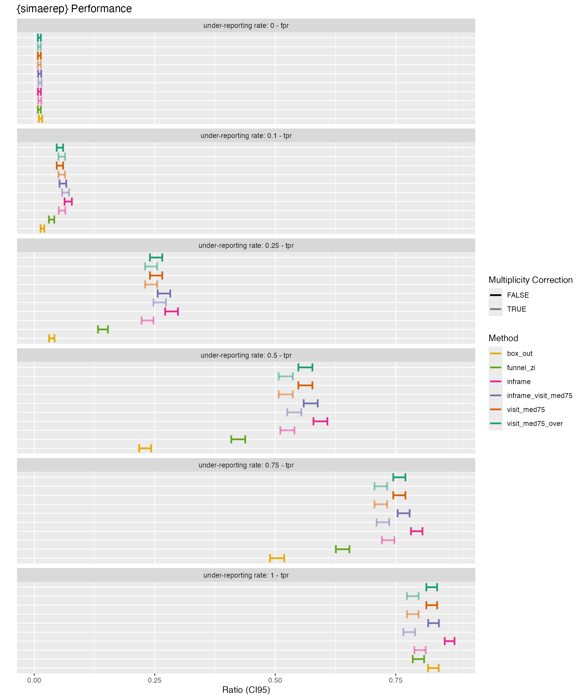

Summary

Multiplicity correction imposes a penalty on the true positive rate

This observation was already made by the Boeringer Ingelheim Team during the evaluation of {simaerep}. We can now reproducibly confirm this. The unaltered probability score as returned by the bootstrap algorithm already provides very realistic under-reporting probabilities.

{simaerep} outperforms simpler methods such as funnel plot and box plot outlier detection.

These controls confirm previous observations that were made during the {simaerep} validation.

{simaerep} algorithm variants are performing more or less at the same level.

The inframe method can be calculated in a database backend and also calculated delta events, while the classic method is faster but requires the data to be processed in memory.