Introduction
With the 0.6.0 release we have added an alternative
version of the {simaerep} algorithm that was coded using solely
dbplyr compatible table operations.
- expand the patients for each site
rtimes - join each patient with a random eligible patient from same study
- for each replicate calculate event per visit rate per site
- calculate the ratio of having a lower event per visit rate than actually observed
This comes with the following advantages and disadvantages:
- Patients are individually matched with patients that have reached the same visit in the study. No need to pick visit_med75 as an evaluation point.
-
dbplyrcompatibility means that code execution can be done in a database back-end as opposed to in-memory. - Matching patients individually is more costly, this increases in-memory computation time
- Limited patient sample pool for patients that have more visits than other patients in study.
Sample Data
set.seed(1)

df_visit <- sim_test_data_study(
  n_pat = 1000, # number of patients in study
  n_sites = 100, # number of sites in study
  frac_site_with_ur = 0.05, # fraction of sites under-reporting
  ur_rate = 0.4, # rate of under-reporting
  ae_per_visit_mean = 0.5 # mean AE per patient visit
)

df_visit$study_id <- "A"
Patient-Level Matching
Here we use the standard version of the algorithm.
To use the patient-level matching algorithm we set
inframe=TRUE and visit_med75=FALSE.
The original algorithm uses fixed seeds before sampling while the inframe method does not. In order to obtain consistent results we need to manually set a seed.
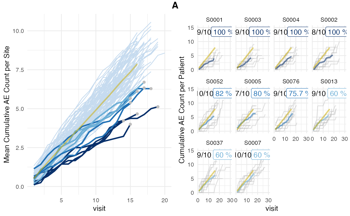
The plot shows that for all sites 10/10 patients were used and none were excluded. We also observe that the site average has become more noisy as less patients are used to calculate the averages for the higher visit numbers.
plot(aerep_inframe)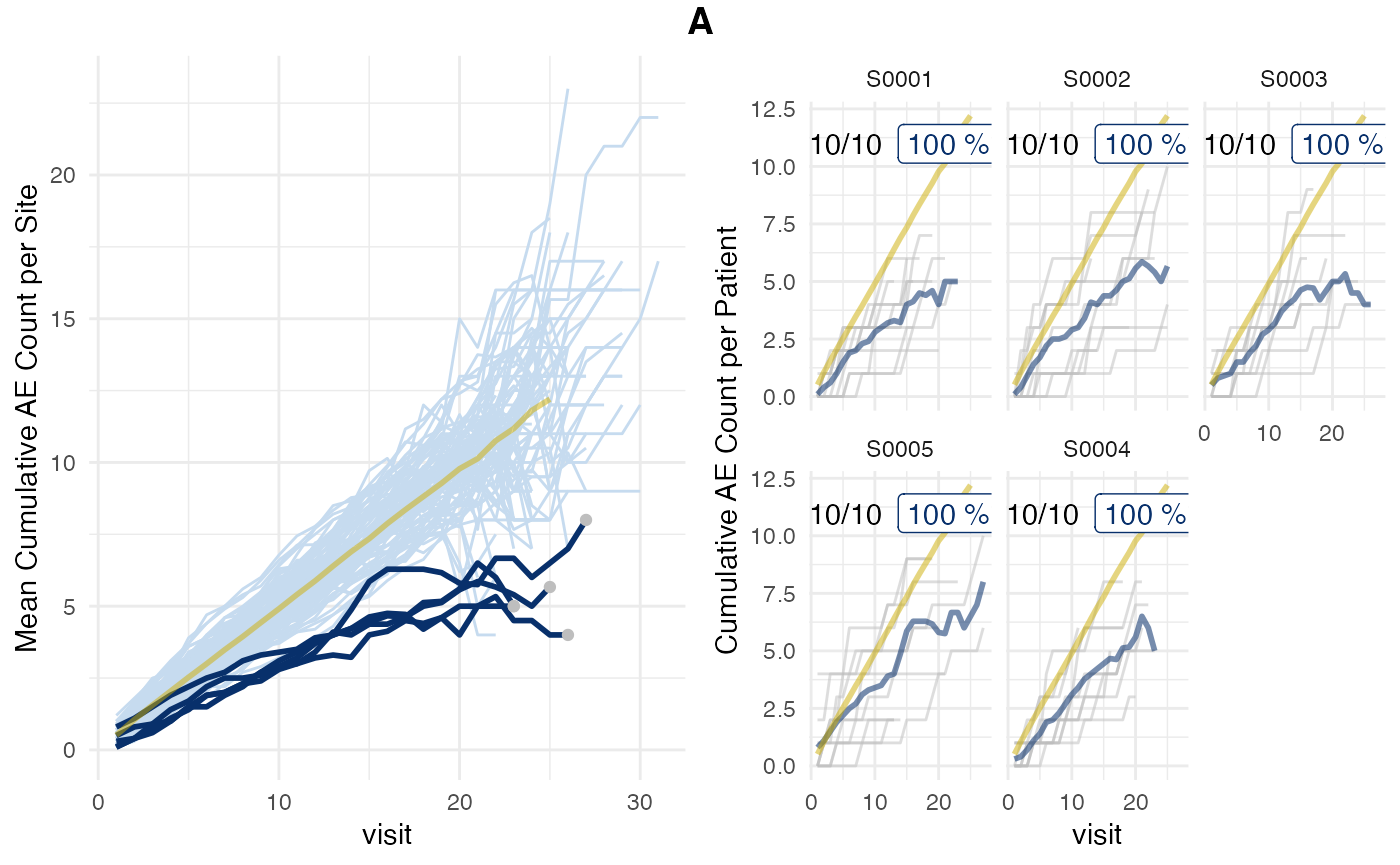
The inframe method includes this noisier data but does not compare
average event counts but event per visit rates. We can find
events_per_visit_site and
events_per_visit_study in df_eval. The latter
is the average event rate obtained in the simulation in which each
patient has been resampled according to its maximum visit.
aerep_inframe$df_eval## # A tibble: 100 × 10
## study_id site_number events events_per_visit_site visits n_pat
## <chr> <chr> <dbl> <dbl> <dbl> <int>
## 1 A S0001 50 0.279 179 10
## 2 A S0002 59 0.281 210 10
## 3 A S0003 55 0.291 189 10
## 4 A S0004 59 0.312 189 10
## 5 A S0005 58 0.297 195 10
## 6 A S0006 100 0.493 203 10
## 7 A S0007 89 0.408 218 10
## 8 A S0008 95 0.559 170 10
## 9 A S0009 101 0.518 195 10
## 10 A S0010 87 0.470 185 10
## # ℹ 90 more rows
## # ℹ 4 more variables: events_per_visit_study <dbl>, prob_low <dbl>,
## # prob_low_adj <dbl>, prob_low_prob_ur <dbl>We can also force the inframe method to use the visit_med75 this will
pre-filter df_visit, which adds an extra step and decreases
performance.
set.seed(1)

aerep_inframe_visit_med75 <- simaerep(
  df_visit,
  inframe = TRUE,
  visit_med75 = TRUE
)

plot(aerep_inframe_visit_med75)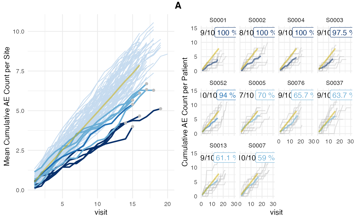
Calculate Reporting Probabilities for Multiple Event Types
We can also calculate the reporting probabilities for multiple event
types. This is done by passing a list of event types to the
event_names parameter.
df_visit <- sim_test_data_study(
  event_names = c("ae", "pd"),
  ae_per_visit_mean = c(0.5, 0.4)
)

df_visit$study_id <- "A"

df_visit %>%
  head(5) %>%
knitr::kable()| patnum | site_number | is_ur | max_visit_mean | max_visit_sd | ae_per_visit_mean | pd_per_visit_mean | visit | n_ae | n_pd | study_id |
|---|---|---|---|---|---|---|---|---|---|---|
| P000001 | S0001 | FALSE | 20 | 4 | 0.5 | 0.4 | 1 | 1 | 1 | A |
| P000001 | S0001 | FALSE | 20 | 4 | 0.5 | 0.4 | 2 | 2 | 1 | A |
| P000001 | S0001 | FALSE | 20 | 4 | 0.5 | 0.4 | 3 | 2 | 1 | A |
| P000001 | S0001 | FALSE | 20 | 4 | 0.5 | 0.4 | 4 | 2 | 1 | A |
| P000001 | S0001 | FALSE | 20 | 4 | 0.5 | 0.4 | 5 | 2 | 1 | A |
eventrep <- simaerep(df_visit, event_names = c("ae", "pd"), inframe = TRUE, visit_med75 = FALSE)

eventrep$df_eval %>%
  select(site_number, starts_with("ae_")) %>%
  head(5) %>%
knitr::kable()| site_number | ae_events | ae_per_visit_site | ae_per_visit_study | ae_prob_low | ae_prob_low_adj | ae_prob_low_prob_ur |
|---|---|---|---|---|---|---|
| S0001 | 456 | 0.4835631 | 0.4999226 | 0.249 | 0.7323077 | 0.2676923 |
| S0002 | 511 | 0.5350785 | 0.5112042 | 0.842 | 0.9273684 | 0.0726316 |
| S0003 | 458 | 0.4751037 | 0.4991961 | 0.147 | 0.7323077 | 0.2676923 |
| S0004 | 480 | 0.4994797 | 0.5010447 | 0.476 | 0.7323077 | 0.2676923 |
| S0005 | 489 | 0.4817734 | 0.4995084 | 0.233 | 0.7323077 | 0.2676923 |
| site_number | pd_events | pd_per_visit_site | pd_per_visit_study | pd_prob_low | pd_prob_low_adj | pd_prob_low_prob_ur |
|---|---|---|---|---|---|---|
| S0001 | 334 | 0.3541888 | 0.3856405 | 0.050 | 0.4600000 | 0.5400000 |
| S0002 | 346 | 0.3623037 | 0.3824126 | 0.155 | 0.6200000 | 0.3800000 |
| S0003 | 386 | 0.4004149 | 0.3879990 | 0.746 | 0.9666667 | 0.0333333 |
| S0004 | 384 | 0.3995838 | 0.3885390 | 0.727 | 0.9666667 | 0.0333333 |
| S0005 | 382 | 0.3763547 | 0.3882680 | 0.279 | 0.6975000 | 0.3025000 |
DB
We can demonstrate the database-backend compatibility by using a
connection to a in memory duckdb database. In order to set
the number of replications we need to create a new table in our back-end
that has one column with as many rows as the desired replications.
A lazy reference to this table can then be passed to the
r parameter.
con <- DBI::dbConnect(duckdb::duckdb(), dbdir = ":memory:")
df_r <- tibble(rep = seq(1, 1000))

dplyr::copy_to(con, df_visit, "visit")
dplyr::copy_to(con, df_r, "r")

tbl_visit <- tbl(con, "visit")
tbl_r <- tbl(con, "r")


aerep <- simaerep(tbl_visit, r = tbl_r, visit_med75 = FALSE)
When inspecting df_eval we see that it is still a lazy
table object.
aerep$df_eval## # Source: SQL [?? x 10]
## # Database: DuckDB v1.2.1 [koneswab@Darwin 23.6.0:R 4.4.1/:memory:]
## # Ordered by: study_id, site_number
## study_id site_number events events_per_visit_site visits n_pat
## <chr> <chr> <dbl> <dbl> <dbl> <dbl>
## 1 A S0007 492 0.489 1006 50
## 2 A S0001 456 0.484 943 50
## 3 A S0003 458 0.475 964 50
## 4 A S0016 467 0.485 962 50
## 5 A S0010 480 0.498 964 50
## 6 A S0004 480 0.499 961 50
## 7 A S0020 503 0.527 955 50
## 8 A S0012 457 0.477 958 50
## 9 A S0005 489 0.482 1015 50
## 10 A S0017 497 0.504 987 50
## # ℹ more rows
## # ℹ 4 more variables: events_per_visit_study <dbl>, prob_low <dbl>,
## # prob_low_adj <dbl>, prob_low_prob_ur <dbl>We can convert it to sql code. The cte option makes the
sql code more readable.
sql_eval <- dbplyr::sql_render(aerep$df_eval, sql_options = dbplyr::sql_options(cte = TRUE))
stringr::str_trunc(sql_eval, 500)
## <SQL> WITH q01 AS (
## SELECT
## patnum,
## site_number,
## is_ur,
## max_visit_mean,
## max_visit_sd,
## ae_per_visit_mean,
## pd_per_visit_mean,
## CAST(visit AS NUMERIC) AS visit,
## CAST(n_ae AS NUMERIC) AS n_ae,
## n_pd,
## study_id
## FROM visit
## ),
## q02 AS (
## SELECT DISTINCT study_id, site_number
## FROM q01
## GROUP BY study_id, site_number, patnum
## ),
## q03 AS (
## SELECT ROW_NUMBER() OVER () AS rep
## FROM r
## ),
## q04 AS (
## SELECT study_id, site_number, patnum, MAX(visit) AS max_visit_per_...We can take that code and wrap it in a CREATE TABLE
statement
## [1] 20Retrieve the new table from the database.
tbl_eval <- tbl(con, "eval")
tbl_eval
## # Source: table<eval> [?? x 10]
## # Database: DuckDB v1.2.1 [koneswab@Darwin 23.6.0:R 4.4.1/:memory:]
## study_id site_number events events_per_visit_site visits n_pat
## <chr> <chr> <dbl> <dbl> <dbl> <dbl>
## 1 A S0006 516 0.493 1047 50
## 2 A S0017 497 0.504 987 50
## 3 A S0016 467 0.485 962 50
## 4 A S0009 508 0.542 937 50
## 5 A S0010 480 0.498 964 50
## 6 A S0003 458 0.475 964 50
## 7 A S0014 493 0.491 1005 50
## 8 A S0015 514 0.511 1006 50
## 9 A S0011 443 0.458 968 50
## 10 A S0007 492 0.489 1006 50
## # ℹ more rows
## # ℹ 4 more variables: events_per_visit_study <dbl>, prob_low <dbl>,
## # prob_low_adj <dbl>, prob_low_prob_ur <dbl>We plot the results from the {simaerep} object.
plot(aerep)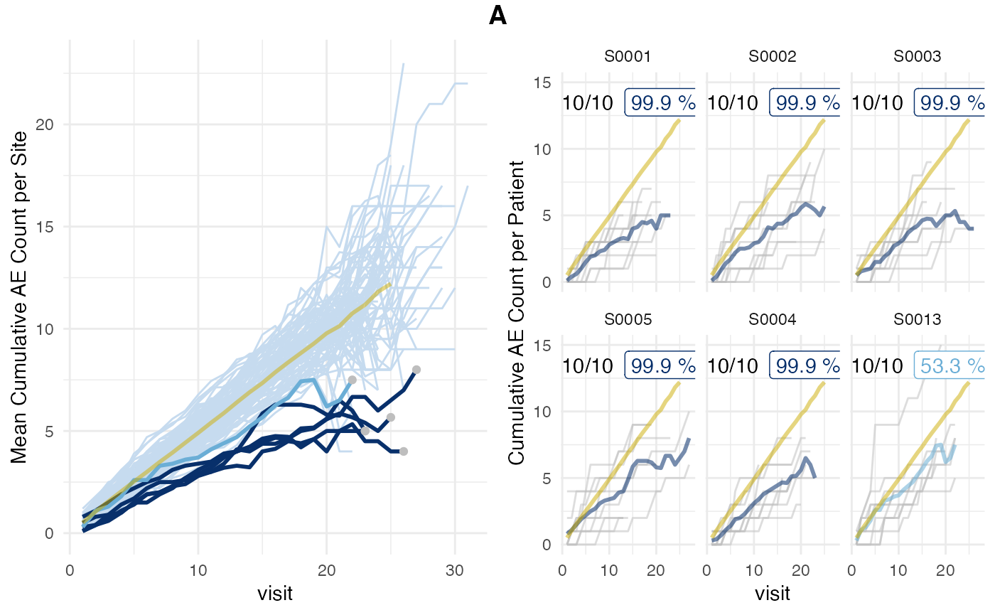
Or more efficiently by using plot_study() when we have
already written the simaerep results into the database.
Here we avoid that the results are being recalculated just for the sake
of creating a plot. However this requires that we save
df_site to the database as well.
sql_site <- dbplyr::sql_render(aerep$df_site)
DBI::dbExecute(con, glue::glue("CREATE TABLE site AS ({sql_site})"))
## [1] 20
tbl_site <- tbl(con, "site")

plot_study(tbl_visit, tbl_site, tbl_eval, study = "A")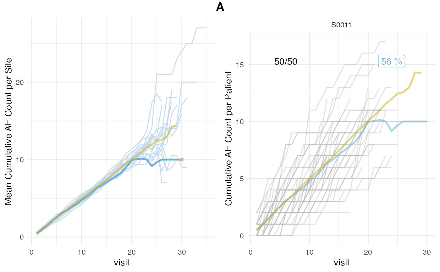
DBI::dbDisconnect(con)In Memory Calculation Times
Here we perform some examplary tests to illustrate the increase in-memory calculation time of the inframe calculation method.
This is the calculation time for the default settings
system.time({simaerep(df_visit, inframe = FALSE, visit_med75 = TRUE, under_only = TRUE, progress = FALSE)})## user system elapsed
## 0.310 0.004 0.315inframe calculation time is higher
system.time({simaerep(df_visit, inframe = TRUE, visit_med75 = FALSE, under_only = TRUE)})## user system elapsed
## 0.701 0.039 0.739