LogisticLogNormalMixture — LogisticLogNormalMixture-class • crmPack

LogisticLogNormalMixture is the class for standard logistic model with online mixture of two bivariate log normal priors.

Usage

LogisticLogNormalMixture(mean, cov, ref_dose, share_weight)

.DefaultLogisticLogNormalMixture()

Arguments

mean: (numeric)
the prior mean vector.
cov: (matrix)
the prior covariance matrix. The precision matrix prec is internally calculated as an inverse of cov.
ref_dose: (number)
the reference dose $x*$ (strictly positive number).
share_weight: (proportion)
the prior weight for the share component.

Details

This model can be used when data is arising online from the informative component of the prior, at the same time with the data of the trial of main interest. Formally, this is achieved by assuming that the probability of a DLT at dose $x$ is given by $$p(x) = \pi * p1(x) + (1 - \pi) * p2(x)$$ where $\pi$ is the probability for the model $p(x)$ being the same as the model $p1(x)$, which is the informative component of the prior. From this model data arises in parallel: at doses xshare, DLT information yshare is observed, in total nObsshare data points (see DataMixture). On the other hand, $1 - \pi$, is the probability of a separate model $p2(x)$. Both components have the same log normal prior distribution, which can be specified by the user, and which is inherited from the LogisticLogNormal class.

Slots

share_weight: (proportion)
the prior weight for the share component $p_{1}(x)$.

Note

Typically, end users will not use the .DefaultLogNormalMixture() function.

Examples

# Decide on the dose grid and MCMC options.
dose_grid <- 1:80
my_options <- McmcOptions()

# Classic model.
my_model <- LogisticLogNormal(
  mean = c(-0.85, 1),
  cov = matrix(c(1, -0.5, -0.5, 1), nrow = 2),
  ref_dose = 50
)

empty_data <- Data(doseGrid = dose_grid)
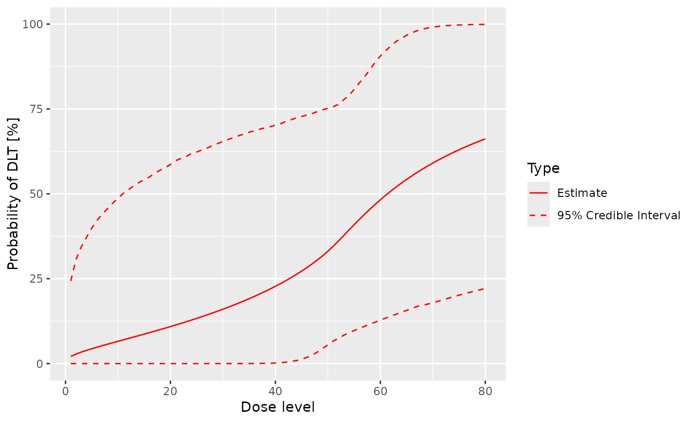
prior_samples <- mcmc(empty_data, my_model, my_options)
plot(prior_samples, my_model, empty_data)


# Set up the mixture model and data share object.
model_share <- LogisticLogNormalMixture(
  share_weight = 0.1,
  mean = c(-0.85, 1),
  cov = matrix(c(1, -0.5, -0.5, 1), nrow = 2),
  ref_dose = 50
)

empty_data_share <- DataMixture(
  doseGrid = dose_grid,
  xshare = rep(c(10, 20, 40), each = 4),
  yshare = rep(0L, 12),
)

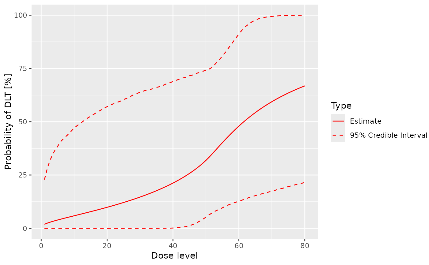
# Compare with the resulting prior model.
prior_samples_share <- mcmc(empty_data_share, model_share, my_options)
plot(prior_samples_share, model_share, empty_data_share)

`LogisticLogNormalMixture`