
Model-based Dose Escalation Designs in R with crmPack (JSS manuscript)
Source:vignettes/crmPack-jss-paper.Rmd
crmPack-jss-paper.RmdAbstract
Model-based dose escalation designs have gained increasing interest
due to the need for more efficient and informative Phase I trials. The
wide-spread implementation of such designs has been hindered by the need
for either licensing specialized commercial software or programming the
design and simulations from scratch for each project. The
R-package crmPack provides a simple and
unified object-oriented framework for model-based dose escalation
designs. This enables the standard use of such designs, while being able
to flexibly adapt and extend them. The framework comprises classes and
methods for the data structure including the dose grid, statistical
models including prior specification, rules for maximum increments, next
best dose, and adaptive stopping and cohort sizes. In addition to
multiple modified classic continual reassessment method and escalation
with overdose control designs with possibly advanced prior
specifications (e.g., minimal informative and mixture priors),
crmPack currently features dual-endpoint (safety and
biomarker) designs and two-part designs. Optional assignment of a small
number of patients in each cohort to placebo instead of treatment
enables the use in trials outside Oncology.
Keywords: continual reassessment method, model based dose escalation, dual-endpoint design, R, object oriented.
Introduction
Phase I trials that are testing new investigational agents in humans for the first time escalate from low to high doses in a sequential fashion. This dose escalation design is necessary in order to reduce the risk of too high and therefore too toxic doses for the probands. These can either be healthy volunteers (e.g., in neurology) or patients (e.g., in oncology), and we will henceforth use only the latter for ease of presentation. While higher doses of agents are usually expected to deliver stronger pharmacodynamic effects and hence improved efficacy, higher doses also usually cause more severe adverse events in the patients. In order to simplify the decision making usually binary dose-limiting toxicities (DLTs) are defined (e.g., adverse events reaching specific severity levels) before starting the trial. The maximum tolerated dose (MTD) is then defined as the dose with a certain probability of DLTs (either using a single value, e.g., 33%, or a range, e.g., 20 to 35%). Historically, patients were treated at the same dose in cohorts of three, with the dose for the next cohort then being determined from the number of DLTs having been observed in the current cohort.
Algorithmic designs like the simple 3+3 design (Carter 1973) have disadvantages that have been recognized in the statistics community, see e.g., (Paoletti et al. 2015). Fundamentally, the escalation rules of the 3+3 design do not have any statistical justification (Storer 1989) in terms of estimating an MTD. Moreover, they cannot be extended to address today’s Phase I trials, with extension cohorts, dose escalation of drug combinations and optimal biological dose determination, naming just a few prominent challenges. Hence model-based dose escalation designs like the continual reassessment method (CRM) (O’Quigley et al. 1990) have gained increasing interest due to the need for more efficient and informative Phase I trials. These designs are based in statistical inference, with dose-toxicity regression models as the backbone, and are therefore flexible for adaptation to various complex trial designs. Importantly, they avoid fixing only a few dose levels in advance. For a wider comparison of algorithmic and model based designs see e.g., (Jaki et al. 2013).
However, the wide-spread implementation of such designs has been
hindered by the need for either licensing specialized commercial
software (thus losing flexibility) or programming the design and
simulations from scratch for each project (thus losing efficiency).
While the models underlying most model-based dose escalation procedures
can easily be fit in standard software with the capability to fit
generalized linear models, e.g., PROC MIXED in
SAS ( Institute Inc. 2003),
glm in Stata (StataCorp
2015) or R ( Core Team
2016), there are still only few software solutions available
dedicated to dose escalation studies.
The commercial packages East (Cytel Inc. 2016) and ADDPLAN (Consultants 2025) both offer extensions to
their basic design software for dose escalation studies
(ESCALATE in East and df in
ADDPLAN) implementing the algorithmic 3+3 design and
various versions of the CRM. Similarly FACTS (Team 2015) also offers different common dose
escalation methods. Due to the commercial nature of these
implementations there is, however, a limitation on how much the designs
can be tailored towards the individual needs of the study. Similarly
static implementations of methods for dose escalation are available in
the Stata module crm (Mander 2013) which implements the CRM and the
dfcrm package (Cheung 2013)
in R which additionally implements the time-to-event CRM
(TITE-CRM) (Cheung and Chappell 2000).
Several R-packages with extensions are available. The
bcrm package (Sweeting et al.
2013) implements a variety of one and two parameter models, and
facilitates different ways to specify prior distributions, escalation
and stopping rules. The ordcrm package (Dressler and Huang 2016) implements ordinal
proportional odds and continuation ratio models for CRMs. The
dfpk package (Toumazi et al.
2017) uses pharmacokinetic data in the dose escalation.
In this paper we introduce the R-package
crmPack (Sabanés Bové et al.
2018) for dose escalation studies, which is publicly available on
CRAN. While the package’s name pays tribute to the original CRM as the
first model-based dose escalation design, the package’s functionality
differs from the above existing implementations in three fundamental
ways. Firstly, it is written using S4 classes and methods
(Chambers 2008), which allows customized
methodology to be added to the package while still being able to use the
existing backbone functionalities. Secondly, methods for studies with a
placebo group (e.g., for healthy volunteer studies) are readily
implemented. Thirdly, dual endpoint dose escalation methods that
incorporate both safety and efficacy and allow determination of an
optimal biological dose are already available.
Framework
For describing the framework of the package we will adapt the general notation for early phase trials from (Thall 2010). Figure @ref(fig:schematic) summarizes the framework in a schematic.
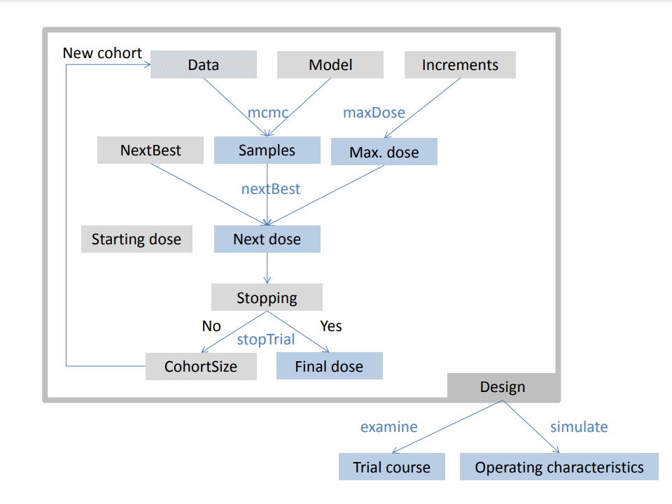
Schematic of the framework
Separate design features are implemented as classes (shown as gray
boxes) and bundled together in the overarching Design
object. They can be processed with various methods (blue text) to run
the dose escalation trial and produce results (blue boxes). For example,
the Data and GeneralModel objects can be
processed by the mcmc method in order to obtain posterior
samples of the model parameters, and given the sample size and the dose
for the next cohort, the updated Data closes the dose
escalation loop. On the higher level, designs can be investigated with
the examine and simulate methods to obtain
hypothetical trial courses and operating characteristics, respectively.
Note that individual model classes and methods are not shown here for
clarity, please refer to the package documentation for details, e.g., by
calling crmPackHelp().’
Data Let denote one specific treatment, chosen from the set of possible treatments ${\cal X}$. This could be one specific dose, but also more generally a vector, containing for example doses of multiple drugs in a combination trial. After giving treatment to a patient, the outcome is observed, typically a safety endpoint as e.g., the binary DLT . Grouping together patients in cohort , generating the cohort data ${\cal C}_{j} = \{(x_{j}, y_{j,1}), \dotsc, (x_{j}, y_{j,n_{j}})\}$, we can denote the data generated from the first cohorts as ${\cal D}_{N}= {\cal C}_{1} \cup \dotsb \cup {\cal C}_{N}$.
In crmPack the S4 class
GeneralData encapsulates this notion and subclasses
implement concrete data structures.
Model The core of model-based dose escalation
designs is the underlying statistical model. Taking a Bayesian approach
to inference, the model in crmPack consists of firstly the
likelihood, which is either a probability density function
or a probability mass function
of
for a patient who receives treatment
assuming the parameter (vector)
,
(this is the likelihood of
)
and secondly the prior
for
given fixed hyperparameters
.
In crmPack the virtual S4 class
GeneralModel encapsulates this notion and subclasses
implement concrete models.
For example, the class LogisticLogNormal implements the
logistic regression model (Neuenschwander et al.
2008) with
parameter vector
,
dose
and specified reference dose
.
The prior
is specified via a bivariate normal distribution on a transformation of
to ensure
:
with hyperparameters
consisting of the prior mean vector
and the prior covariance matrix
.
Decision making for the next dose Another core element of a dose escalation design concerns the decision making for the next dose to be tested in the next cohort . In the (Thall 2010) notation, the function is mapping the currently accumulated data to the dose space (or to dose , meaning to stop the trial because all doses are too toxic): $$\begin{equation} \alpha: {\cal D}_{N} \rightarrow \mathcal{X} \cup \{0\} \end{equation}$$ This mapping is commonly specified via the combination of two elements: The first element is a function for the maximum increments between dose levels, which can calculate from the current data (including the current dose ) the maximum possible next dose for the next cohort. The second element is a rule indirectly acting on the current data through the posterior distribution and the maximum possible dose to finally give the next dose .
In crmPack maximum increments are specified by
subclasses of Increments, and the next best dose rule by
subclasses of NextBest.
The design class Additional features of a design
concern the adaptive sizing of the next cohort and the adaptive stopping
of the trial. Those are implemented in subclasses of
CohortSize and Stopping, respectively.
Moreover, the starting dose
is also a feature of the design.
Finally, the overall dose escalation design is bundling all the
described features together in a dedicated class typically inheriting
from Design.
As noted in (Thall 2010), the operating
characteristics of such a complex dose escalation design can only be
evaluated by simulations. This can be done using the
simulate methods for the design classes, and is recommended
to be performed for a multitude of different scenarios in order to
stress-test the design and to convince oneself of its properties.
In particular, the operating characteristics reveal whether the MTD can be estimated well by the designs.
In addition, the examine method evaluates hypothetical
trial outcomes and lists the resulting trial decisions (dose for the
next cohort and trial end).
In order to illustrate the use of this object-oriented framework, the next section contains practical examples on use of the existing functionality as well as an example for creating new extensions.
Using crmPack
We consider a trial in Type II diabetes carried out by Hoffmann-La
Roche Ltd. in order to illustrate the functionality in the package. For
each patient, we observed a binary safety (DLT) and a continuous
efficacy outcome. In Implementing a
CRM trial we will show how to implement a CRM design for dose
escalation based on the safety endpoint only, while in Dose escalation with
safety and efficacy also the efficacy endpoint will be considered.
Extending crmPack
functionality gives an example on extending the crmPack
functionality.
Before we start, we have to install and subsequently load our package
in R:
As indicated in the startup message, try
crmPackHelp()andcrmPackExample()to open the help page and the package vignette.
Implementing a CRM trial
Suppose that 12 dose levels ranging from 25 to 300 mg in 25 mg increments of a novel agent are available in addition to placebo, defining our dose grid , with mg representing placebo and being our starting dose. Note that here we used a very small dose instead of zero for , since we consider here the regression model @eqref(eq:LogisticLogNormal) with a log transformation of the dose (with chosen as reference dose).
Minimally informative prior Here we assume that
limited prior information is available on the dose-toxicity
relationship, and hence would like to use a minimally informative prior
(Neuenschwander et al. 2008) which can be
easily obtained with the function MinimalInformative. Since
stochastic optimization is used internally, setting of a seed is
required for reproducibility. Furthermore, it is recommended to specify
a coarse dose grid across the original dose range (excluding the placebo
dose) to avoid long computation time:
coarseGrid <- c(25, 50, 100, 200, 300)
model <- MinimalInformative(
  dosegrid = coarseGrid, refDose = 100,
  logNormal = TRUE, threshmin = 0.1,
  threshmax = 0.2, seed = 432,
  control = list(max.time = 30)
)$model
The resulting model (which is an object of class
LogisticLogNormal) has prior parameters
and
and will
approximately have 5% probability each for the DLT rate to exceed 10%
(threshmin argument) at the 25 mg dose and to be below 20%
(threshmax) at the 300 mg dose.
Data object definition and visualization In this
simple case of a univariate dose
resulting in binary DLT observations
,
the S4 class Data can be used. Objects of this
class can be created by calling the accompanying initialization function
of the same name (which is a general convention in
crmPack):
PL <- 0.001
data <- Data(
  x = c(PL, 25, 25, 25, PL, 50, 50, 50, PL, 100, 100, 100),
  y = c(0, 0, 0, 0, 0, 0, 0, 0, 0, 0, 1, 0),
  cohort = c(1, 1, 1, 1, 2, 2, 2, 2, 3, 3, 3, 3),
  doseGrid = c(PL, seq(25, 300, 25)),
  ID = 1:12,
  placebo = TRUE
)
The argument x takes the doses
(note the repetition to match the outcome variables
)
where doseGrid captures the set ${\cal X}$ of all possible doses,
y takes the binary DLTs (here
denotes the only DLT having been observed in the 3rd patient in the 3rd
cohort), while cohort groups the patients together in
cohorts (here
).
The option placebo is used to specify that this is a
placebo controlled study, with placebo patients included in each cohort.
The lowest dose
is then interpreted internally as the placebo dose. Patient IDs can be
given optionally in the ID argument. The data can then be
visualized by simply applying the plot function to the
object, which also allows to produce a blinded plot (hiding patient IDs
and placebo/treatment assignment) with the option blind,
see Figure @ref(fig:plot-data):
plot(data)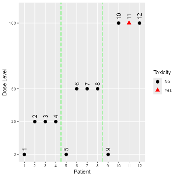
Open and blinded data plots
plot(data, blind = TRUE)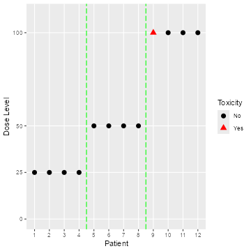
Open and blinded data plots
Sampling from the prior and posterior Now that we
have the model and the data in place, we can use MCMC sampling for
obtaining the posterior distribution of the model parameters
,
and hence the DLT rates
,
at various doses
.
The MCMC sampling can be controlled with an object of class
McmcOptions, which is then provided to the
mcmc function, together with the data and the
model objects:
options <- McmcOptions(burnin = 1000, step = 2, samples = 10000)
set.seed(94)
samples <- mcmc(data, model, options)
The posterior mean curve and 95% equi-tailed credible interval curves
for the DLT rates can be obtained by supplying the samples, model and
data to the generic plot function. Similarly we can also
produce a similar plot without any data, which is then giving the prior,
see Figure @ref(fig:plot-model-fit):
plot(samples, model, data) + ggtitle("Posterior")

emptydata <- Data(doseGrid = data@doseGrid, placebo = TRUE)
priorsamples <- mcmc(emptydata, model, options)
plot(priorsamples, model, emptydata) + ggtitle("Prior")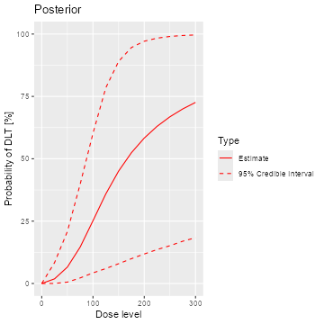
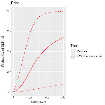
Posterior and prior regression model fits
As illustrated here, the plots can be customized by using the
ggplot2(Wickham 2009)
functionality. We can see that while the posterior mean estimate (left
panel, continuous line) is only slightly steeper than the prior mean
estimate curve (right panel, continuous line), the posterior uncertainty
is reduced due to the data (smaller credible intervals, dashed
lines).
Decision making for the next dose To determine which
dose to administer to the next (cohort of) patients we begin by
specifying the maximum increments function
.
In the example below a maximum increase of 100% for doses below 100 mg,
50% for doses in the range from 100 mg to 200 mg, and 33% for doses
equal or above 200 mg is specified using the class
IncrementsRelative:
myIncrements <- IncrementsRelative(
  intervals = c(0, 100, 200),
  increments = c(1, 0.5, 0.33)
)
This specific rule
can then be evaluated on the current dataset ${\cal D}_{N}$ by the maxDose
function to obtain the maximum next dose $t_{N+1} = \tau({\cal D}_{N})$:
(nextMaxDose <- maxDose(myIncrements, data))
#> [1] 150
We then define the function
for selecting a dose for the next cohort. In this case we would like to
select the dose which maximizes the probability of the DLT rate being in
the target toxicity range from 20% to 35%, but with the probability of
overdosing not exceeding 25% (Neuenschwander et
al. 2008), using the NextBestNCRM class:
myNextBest <- NextBestNCRM(
  target = c(0.2, 0.35), overdose = c(0.35, 1),
  max_overdose_prob = 0.25
)
This rule can then be evaluated with the function
NextBest to obtain the next dose $x_{N+1}=\nu({\cal D}_{N}, t_{N+1})$:
nextDoseRes <- nextBest(myNextBest, nextMaxDose, samples, model, data)
(nextDoseVal <- nextDoseRes$value)
#> [1] 100
The returned list also contains an accompanying plot
(nextDoseRes$plot), see Figure @ref(fig:nextBest-ncrm).
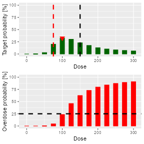
Dose recommendation plot from NCRM design
Adaptive stopping of the trial We would like to stop
the dose escalation adaptively if the maximum sample size of
patients has been reached already, or if we have sufficient precision
for the MTD estimate. We can specify the latter condition as follows:
The probability that the next dose
is in the target toxicity range is above 50%, and at least 9 patients
were already dosed within +/- 20% range of
.
The corresponding Stopping class object is constructed by
combining the atomic rules with logical operators as follows:
myStopping1 <- StoppingMinPatients(nPatients = 30)
myStopping2 <- StoppingTargetProb(target = c(0.2, 0.35), prob = 0.5)
myStopping3 <- StoppingPatientsNearDose(nPatients = 9, percentage = 20)
myStopping <- myStopping1 | (myStopping2 & myStopping3)
Again, this specific rule can be evaluated by a function, here called
stopTrial, for a specific situation:
stopTrial(myStopping, nextDoseVal, samples, model, data)
#> [1] FALSE
#> attr(,"message")
#> attr(,"message")[[1]]
#> [1] "Number of patients is 12 and thus below the prespecified minimum number 30"
#>
#> attr(,"message")[[2]]
#> attr(,"message")[[2]][[1]]
#> [1] "Probability for target toxicity is 33 % for dose 100 and thus below the required 50 %"
#>
#> attr(,"message")[[2]][[2]]
#> [1] "3 patients lie within 20% of the next best dose 100. This is below the required 9 patients"
#>
#>
#> attr(,"individual")
#> attr(,"individual")[[1]]
#> [1] FALSE
#> attr(,"message")
#> [1] "Number of patients is 12 and thus below the prespecified minimum number 30"
#> attr(,"report_label")
#> [1] "≥ 30 patients dosed"
#>
#> attr(,"individual")[[2]]
#> [1] FALSE
#> attr(,"message")
#> attr(,"message")[[1]]
#> [1] "Probability for target toxicity is 33 % for dose 100 and thus below the required 50 %"
#>
#> attr(,"message")[[2]]
#> [1] "3 patients lie within 20% of the next best dose 100. This is below the required 9 patients"
#>
#> attr(,"individual")
#> attr(,"individual")[[1]]
#> [1] FALSE
#> attr(,"message")
#> [1] "Probability for target toxicity is 33 % for dose 100 and thus below the required 50 %"
#> attr(,"report_label")
#> [1] "P(0.2 ≤ prob(DLE | NBD) ≤ 0.35) ≥ 0.5"
#>
#> attr(,"individual")[[2]]
#> [1] FALSE
#> attr(,"message")
#> [1] "3 patients lie within 20% of the next best dose 100. This is below the required 9 patients"
#> attr(,"report_label")
#> [1] "≥ 9 patients dosed in 20 % dose range around NBD"
#>
#> attr(,"report_label")
#> [1] NA
#>
#> attr(,"report_label")
#> [1] NA
The result FALSE means that we cannot yet stop the
trial, with the attribute message giving the results from
the atomic stopping rules.
Examine the dose escalation design In the last topic
of this section, we want to show how to assess the performance of a
given CRM design. We first need to specify our design by creating an
object of class Design. It contains our model, our rules
for dose escalation (Increments, NextBest,
Stopping and CohortSize), the dose grid (in
the example below through the object emptydata) and our
starting dose (see also Figure @ref(fig:schematic). In this case we will
use a fixed cohort size of 3 patients on active and 1 patient on placebo
(``3+1’’) throughout the study:
mySize <- CohortSizeConst(3)
mySizePL <- CohortSizeConst(1)

design <- Design(
  model = model, nextBest = myNextBest,
  stopping = myStopping, increments = myIncrements,
  cohort_size = mySize, pl_cohort_size = mySizePL,
  data = emptydata, startingDose = 25
)
We can then start by looking at the single trial operating
characteristics of the dose escalation design with the function
examine, which generates a data frame showing the beginning
of several hypothetical trial courses under the design. Assuming no DLTs
have been seen until a certain dose, then the consequences of different
number of DLTs being observed at this dose are shown. For example, if we
observe 3 DLTs at the starting dose of 25 mg, we would need to stop the
trial, while we would enroll another cohort at the same dose level in
case of 2 DLTs. In the last rows of the output we see that if no DLTs
were observed before the 250 mg cohort, the maximum considered dose of
300 mg dose can be reached in the next cohort if also no DLTs are
observed at 250 mg. If 1, 2 or 3 DLTs are observed, the next dose is
recommended as 225, 175 and 150 mg, respectively.
set.seed(23)
examine(design, mcmcOptions = options)
#>    dose DLTs nextDose  stop increment
#> 1    25    0       50 FALSE       100
#> 2    25    1       50 FALSE       100
#> 3    25    2       25 FALSE         0
#> 4    25    3       NA FALSE        NA
#> 5    50    0      100 FALSE       100
#> 6    50    1       75 FALSE        50
#> 7    50    2       50 FALSE         0
#> 8    50    3       25 FALSE       -50
#> 9   100    0      125 FALSE        25
#> 10  100    1      100 FALSE         0
#> 11  100    2       75 FALSE       -25
#> 12  100    3       50 FALSE       -50
#> 13  125    0      175 FALSE        40
#> 14  125    1      125 FALSE         0
#> 15  125    2      100 FALSE       -20
#> 16  125    3       75 FALSE       -40
#> 17  175    0      250 FALSE        43
#> 18  175    1      175 FALSE         0
#> 19  175    2      125 FALSE       -29
#> 20  175    3      100 FALSE       -43
#> 21  250    0      300 FALSE        20
#> 22  250    1      225 FALSE       -10
#> 23  250    2      175 FALSE       -30
#> 24  250    3      150 FALSE       -40
Simulating operating characteristics For the many
trials operating characteristics, we first have to define true
scenarios, from which the data should arise. In this case, this only
requires a function that computes the probability of DLT given a dose.
As an example we use here the function contained in the slot
prob of the object model: %, for which the
dose-toxicity curve is shown below.
myTruth <- probFunction(model, alpha0 = 4.5, alpha1 = 8)Note that any possible R-function returning a vector of probabilities upon input of the dose vector can be used. In particular, it is trivially possible to directly specify the probability of DLT for each dose in order to examine operating characteristics not based on any statistical model. For example, assume 5 doses 1–5 with probabilities of DLT of 0.01, 0.02, 0.04, 0.06, 0.09, then the following code could be used:
doseProbMatrix <- cbind(c(1, 2, 3, 4, 5), c(0.01, 0.02, 0.04, 0.06, 0.09))
myTruthMatrix <-
  function(dose) {
    doseProbMatrix[match(dose, doseProbMatrix[, 1]), 2]
  }
Now we can proceed to the simulations using the function
simulate:
mySimsTime <-
  system.time(mySims <- simulate(design,
    truth = myTruth, nsim = 100,
    seed = 819, mcmcOptions = options,
    parallel = FALSE
  ))[3]
The number of simulated trials depends on the required accuracy of
the results. The argument parallel can be set to
TRUE if one wishes to run the iterations in parallel on all
processors of the computer, which can yield a meaningful speedup. Here
we needed 274 seconds for 100 simulated trials on an Intel Core i5-6300U
CPU with 2.4 GHz.
The result is an object of class Simulations containing
multiple slots, with e.g., the data slot containing the
list of simulated trials. The slots doses and
stopReasons contain information about the final MTD and the
stopping reason for each trial. We can e.g., investigate the number of
patients and the MTD at the end of the third simulated trial:
mySims@data[[3]]@nObs
#> [1] 32
mySims@doses[3]
#> [1] 25Simulations object by calling
the plot method on it, see Figure @ref(fig:sim-plot). You
can select the plots by changing the type argument of
plot, which by default is
type = c("trajectory", "dosesTried").
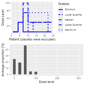
Simulation plot
Second, we can summarize the simulation results, and obtain a textual description of the results:
simSum <- summary(mySims, truth = myTruth)
simSum
#> Summary of 100 simulations
#>
#> Target toxicity interval was 20, 35 %
#> Target dose interval corresponding to this was 47.9, 52.7
#> Intervals are corresponding to 10 and 90 % quantiles
#>
#> Number of patients on placebo : mean 7 (6, 8)
#> Number of patients on active : mean 22 (18, 24)
#> Number of patients overall : mean 30 (24, 32)
#> Number of patients treated above target tox interval : mean 3 (0, 3)
#> Proportions of DLTs in the trials for patients on placebo : mean 0 % (0 %, 0 %)
#> Proportions of DLTs in the trials for patients on active : mean 28 % (21 %, 38 %)
#> Mean toxicity risks for the patients on active : mean 27 % (18 %, 33 %)
#> Doses selected as MTD : mean 46 (25, 50)
#> True toxicity at doses selected : mean 22 % (0 %, 26 %)
#> Proportion of trials selecting target MTD: 84 %
#> Dose most often selected as MTD: 50
#> Observed toxicity rate at dose most often selected: 27 %
#> Fitted toxicity rate at dose most often selected : mean 23 % (16 %, 30 %)
#> Stop reason triggered:
#>  ≥ 30 patients dosed :  65 %
#>  P(0.2 ≤ prob(DLE | NBD) ≤ 0.35) ≥ 0.5 :  45 %
#>  ≥ 9 patients dosed in 20 % dose range around NBD :  98 %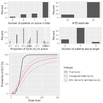
Simulation summary plot
Dose escalation with safety and efficacy
In this section, dose escalation designs incorporating both safety
(as binary DLT) and efficacy endpoints (continuous response) will be
introduced. Dual endpoint datasets are implemented with the
DualData class, where here we illustrate the addition of
the efficacy data w to the previous dataset:
data2 <- DataDual(
  x = data@x, y = data@y, placebo = TRUE,
  w = c(
    0.02, 0.42, 0.59, 0.45, 0.03, 0.7, 0.6, 0.52,
    0.01, 0.71, 0.54, 0.45
  ), cohort = data@cohort,
  doseGrid = data@doseGrid, ID = data@ID
)
The endpoints can be modelled jointly or separately. For joint
modelling derived from (Bekele and Shen
2005), please see the package vignette and the
DualEndpoint class. In the following section we will
describe separate modelling, as proposed in (Yeung et al. 2015). We will show how the dual
endpoint design can help to estimate an optimal dose level which
represents the best trade-off between safety and efficacy.
Methodology Briefly introducing the methodology in current notation, assume that the dose grid $\cal{X}$ contains dose levels, and the logistic regression model @ with is used for the safety endpoint . For the continuous efficacy endpoint , a linear log-log model can be used, conditional on (no DLT): such that with as a constant. Usually the default value can be used, but in our case we choose to allow for the placebo dose which is close to 0.
For both the safety and efficacy models, the prior will be expressed in form of imaginary pseudo data see (Yeung et al. 2015) for details. Prior and posterior modal estimates of the model parameters can then be obtained as the maximum likelihood estimates from the data set combining pseudo data with observed data (Whitehead 2006). The variance can be fixed or assigned an inverse gamma prior distribution.
Model classes The ModelPseudo class
contains all model classes where the priors are specified in terms of
pseudo data, with subclasses for safety (ModelTox) and
efficacy (ModelEff).
Coming back to our example study, the pseudo data for the safety prior assumes that 3 subjects each are treated at the lowest (25 mg) and the highest (300 mg) dose level, with 1.05 and 1.8 DLTs being observed at these two dose levels, respectively. This corresponds to prior means of 0.35 and 0.6 for the DLT probabilities. We implement model @ with this pseudo data prior as follows:
DLTmodel <- LogisticIndepBeta(
  binDLE = c(1.05, 1.8), DLEweights = c(3, 3),
  DLEdose = c(25, 300), data = emptydata
)
The efficacy model can similarly be specified as
emptydata2 <- DataDual(doseGrid = emptydata@doseGrid, placebo = TRUE)
Effmodel <- Effloglog(
  eff = c(1.223, 2.513), eff_dose = c(25, 300),
  nu = c(a = 1, b = 0.025), data = emptydata2, c = 2
)
Here the argument Eff takes the vector of pseudo
efficacy responses at the two fixed dose levels, assuming one subject is
treated at each of these dose levels. The argument nu
specifies a Gamma prior distribution with shape 1 and rate 0.025 for the
precision parameter of the pseudo efficacy responses.
Decision making for the next dose A gain function is
used to quantify the trade-off between efficacy and safety, and the next
dose should maximize the estimated gain modulo safety constraints. Here
we will define the gain as the expected efficacy response, with the
convention that a DLT will automatically lead to a zero efficacy
response:
Note that the gain
function depends on the safety parameter vector
and the efficacy parameters
and
,
which will be estimated by their posterior modal estimates using the
update method:
newDLTmodel <- update(object = DLTmodel, data = data2)
newEffmodel <- update(object = Effmodel, data = data2)
With crmPack we can implement the next best dose
recommendation based on maximizing the gain function as follows:
GainNextBest <- NextBestMaxGain(
  prob_target_drt = 0.35,
  prob_target_eot = 0.3
)
where prob_target_drt specifies the maximum estimated
DLT rate tolerated during the study and prob_target_eot the
maximum estimated DLT rate tolerated at the end of the study. As in Implementing a CRM trial this rule
can be evaluated using NextBest to obtain
,
after evaluating the maximum increments rule
using maxDose to obtain
:
(nextMaxDose <- maxDose(myIncrements, data2))
#> [1] 150
doseRecGain <- nextBest(GainNextBest,
  doselimit = nextMaxDose,
  model = newDLTmodel, model_eff = newEffmodel,
  data = data2
)
(nextDoseVal <- doseRecGain$next_dose)
#> [1] 25doseRecGain$plot and shown in Figure
@ref(fig:doseRecommendation). \begin{figure}
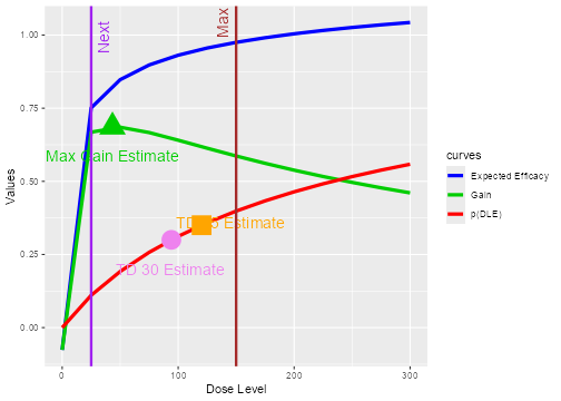
plot of chunk doseRecommendation
Dose recommendation plot from dual endpoint design. The red, blue and
green curves correspond to the (posterior modal) estimated curves for
safety, efficacy and gain, respectively. The vertical red line in the
plot shows the maximum possible dose
mg and the vertical violet line shows the next dose
mg. The circle, square and triangle symbols mark the estimated doses
with target toxicity (100 mg for 35% DLT probability during the trial
and 75 mg for 30% DLT probability at the end of trial) and the estimated
dose with maximum gain, 25 mg. The numbers can be obtained from the
doseRecGain list.
Stopping rules In addition to the simple stopping rule based on the maximum number of patients in our trial, we can use another one relating to the precision of the dose with optimum gain:
myStopping4 <- StoppingMaxGainCIRatio(
  target_ratio = 5,
  prob_target = GainNextBest@prob_target_eot
)
myStoppingDual <- myStopping1 | myStopping4
This stops the trial when 30 patients are reached, or when the ratio of the upper and lower confidence interval bounds around the dose recommendation is less than 5.
Simulations To simulate the operating characteristics, first a design has to be built:
design2 <- DualResponsesDesign(
  nextBest = GainNextBest, model = DLTmodel,
  eff_model = Effmodel, data = emptydata2,
  stopping = myStoppingDual,
  increments = myIncrements,
  cohort_size = mySize, startingDose = 25
)
Note that an additional slot for the efficacy model is included in this design class. We can then specify the scenario for the simulation, by defining the true DLT and efficacy curves that we will be using:
myTruthDLT <- probFunction(DLTmodel, phi1 = -53, phi2 = 10)
myTruthEff <- efficacyFunction(Effmodel, theta1 = -4.8, theta2 = 3.7)
myTruthGain <- function(dose) {
  myTruthEff(dose) * (1 - myTruthDLT(dose))
}
Please note that the parameter names phi1,
phi2, theta1 and theta2
correspond to
and
,
respectively. Simulations are again produced by the
simulate function:
Sim1 <- simulate(
  object = design2, args = NULL, trueDLE = myTruthDLT,
  trueEff = myTruthEff, trueNu = 1 / 0.025, nsim = 20,
  seed = 819, parallel = FALSE
)
Note that the fixed precision nu
is specified instead of the variance
.
% The results of the simulation can then be plotted and summarized as
shown before.
Extending crmPack functionality
One of the big advantages of crmPack over existing
R implementations is its flexible framework based on the
S4 classes and methods system (Chambers 2008) and JAGS (Plummer 2003) for Bayesian computations. Here
we will therefore illustrate how users can extend the existing
functionality easily to the specific needs of the study.
Objective The example will implement a version of the one-parameter CRM (O’Quigley et al. 1990), which is currently not (yet) included in the package. It is based on a one-parameter power model to describe the relationship between the binary DLT responses and their corresponding dose levels : Here is monotonically increasing in and is specified by the investigator upfront. The sequence along the dose grid is often called ``skeleton’’ of the CRM. An exponential distribution with parameter is imposed as the prior distribution for the unknown parameter . The next dose should then be chosen such that the distance of the posterior mean estimated DLT probability to a predefined target toxicity level is minimized.
Creating a new model To implement the one-parameter
model @ in crmPack we first need to define an appropriate
S4 class inheriting from the general model class
GeneralModel:
.OneParExp <- setClass(
  Class = "OneParExp",
  contains = "GeneralModel",
  slots = c(
    skeleton_probs = "numeric",
    dose_grid = "numeric",
    lambda = "numeric"
  )
)
Here we specify that the new class is called OneParExp
and contains three additional slots containing the resulting skeleton
prior probabilities, the dose grid, and the prior parameter
.
Second we have to create a convenient initialization function, which
specifies the likelihood and prior distributions in the underlying
GeneralModel in JAGS. We choose to let the
user supply just the skeleton probabilities along with the intended dose
grid to use. The likelihood with the power model is specified in
datamodel and uses the Data slots which are
specified in datanames. The prior is defined in
priormodel. Model parameters are passed to
JAGS via modelspecs. The init
slot contains a function giving the starting values for the MCMC
sampler, and sample defines which parameter samples will be
returned:
OneParExp <- function(skeleton_probs, dose_grid, lambda) {
  .OneParExp(
    skeleton_probs = skeleton_probs,
    dose_grid = dose_grid,
    lambda = lambda,
    datamodel = function() {
      for (i in 1:nObs) {
        y[i] ~ dbern(p[i])
        p[i] <- skeleton_probs[xLevel[i]]^theta
      }
    },
    priormodel = function() {
      theta ~ dexp(lambda)
    },
    modelspecs = function() {
      list(skeleton_probs = skeleton_probs, lambda = lambda)
    },
    init = function() {
      list(theta = 1)
    }, sample = "theta",
    datanames = c("nObs", "y", "xLevel")
  )
}
Finally, we will create the dose and prob
methods. The prob method is based on the (a skeleton)
function which does the interpolation between the dose grid points in
order to obtain the probability of a DLT. The dose, on the
other hand, uses an inverse of (the skeleton) function
which maps the
probability
to a dose
.
setMethod(
  f = "dose",
  signature = signature(
    x = "numeric",
    model = "OneParExp",
    samples = "Samples"
  ),
  definition = function(x, model, samples) {
    theta <- samples@data$theta
    invSkeletonFun <- approxfun(x = model@skeleton_probs, y = model@dose_grid, rule = 1)
    invSkeletonFun(x^(1 / theta))
  }
)

setMethod(
  f = "prob",
  signature = signature(
    dose = "numeric",
    model = "OneParExp",
    samples = "Samples"
  ),
  definition = function(dose, model, samples) {
    theta <- samples@data$theta
    skeletonFun <- approxfun(x = model@dose_grid, y = model@skeleton_probs, rule = 2)
    skeletonFun(dose)^theta
  }
)
Now we can already use the model, for example in the following we specify the skeleton probabilities via the dose grid and use a standard exponential prior for . The resulting posterior fit can be plotted as usual, see Figure @ref(fig:OneParExp-model-example).
(skeleton_probs <- round(data@doseGrid / max(data@doseGrid) / 2, 2))
#>  [1] 0.00 0.04 0.08 0.12 0.17 0.21 0.25 0.29 0.33 0.38 0.42 0.46 0.50
newModel <- OneParExp(
  skeleton_probs = skeleton_probs,
  dose_grid = data@doseGrid,
  lambda = 1
)
newSamples <- mcmc(data, newModel, options)
plot(newSamples, newModel, data)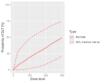
Model fit of the one parameter power model
Creating a new dose recommendation rule In a second
step we would like to create a new dose recommendation rule, which
proposes the dose with estimated DLT probability closest to the target.
Again we start with the class, now inheriting from
NextBest:
.NextBestMinDist <- setClass(
  Class = "NextBestMinDist",
  contains = "NextBest",
  representation(target = "numeric")
)
NextBestMinDist <- function(target) {
  .NextBestMinDist(target = target)
}
Note that here we keep to the convention of separate class definition
and initialization function, although there is no technical need in this
case. In order to make it usable we need to define the
NextBest method for this new rule. Note that we do only
specialize the method for the first argument, such that this rule could
also be used with other models.
setMethod(
  "nextBest",
  signature = signature(
    nextBest = "NextBestMinDist",
    doselimit = "numeric",
    samples = "Samples",
    model = "OneParExp",
    data = "Data"
  ),
  def = function(nextBest, doselimit, samples, model, data, ...) {
    dosesOK <-
      if (length(doselimit)) {
        which(data@doseGrid <= doselimit)
      } else {
        seq_along(data@doseGrid)
      }
    modelfit <- fit(samples, model, data)
    probDLT <- modelfit$middle[dosesOK]
    doses <- modelfit$dose[dosesOK]
    bestIndex <- which.min(abs(probDLT - nextBest@target))
    bestDose <- doses[bestIndex]
    list(value = bestDose)
  }
)
In the method definition, we can use the fit function in
order to obtain the estimated DLT rates. We need to return a
list from this method, since this is required by the
generic function definition. The advantage is that we could also include
a plot or other supporting information in the return value. Immediately
we can now use this rule in order to obtain the next dose
recommendation, e.g., after specifying a target dose of 30%:
newMyNextBest <- NextBestMinDist(target = 0.3)
newNextDoseVal <- nextBest(newMyNextBest, nextMaxDose, newSamples, newModel, data)$value
newNextDoseVal
#> [1] 150
So using this CRM, we could escalate to 150 mg, instead of just 100 mg above.
Using the new functionality These were the only
necessary additions of code that we needed to implement the
one-parameter CRM with a greedy next best dose rule - from now on we can
use the new classes in the same way as classes already contained in
crmPack! For example, we can create a corresponding new
Design object, examine its hypothetical trial course and
run simulations. In particular, the placebo convention automatically
carries over.
Summary
In this paper we have introduced the R package
crmPack for analyzing and evaluating dose escalation
trials. Unlike existing software the package is written to make full use
of a class structure enabling easy extensions to user-specific
dose-response models, prior distributions, escalation and stopping
rules. The example in Extending crmPack
functionality demonstrated that:
- New functionality can be added - without changing the package.
- Only the new functionality needs to be coded in one place - no side effects need to be considered.
- Templates for new designs can be found by looking at the existing
code in the package - only minimal
S4andJAGSknowledge is required.
Therefore, crmPack allows the user to easily extend the
package by keeping modifications local and limited to what needs to be
changed, which in our experience has been a key success factor for the
wider use of model-based dose escalation designs. The package does,
however, already include a wide range of model-based and algorithmic
dose escalation procedures, which are described in the package’s
documentation available through crmPackHelp() and provide
end-users easy access to these approaches without the need for further
coding. Another unique feature of the package is the inclusion of
approaches that allow placebo data, which are routinely collected in
healthy volunteer studies, to be utilized. Finally some methods
[e.g.,](Bekele and Shen 2005)(Yeung et al. 2015) for dose-finding
incorporating safety and efficacy are implemented already in the
package. As for all designs, the underlying structure to extend to novel
dual endpoint methods is provided. Simulation facilities for all
approaches and relevant graphical displays are also available.
The package is actively developed further and new methods will be
added. Future extensions of crmPack will include
model-based combination dose escalation designs, see for example (Sweeting and Mander 2012) and [Riviere et al. (2014) for recent reviews.
Furthermore, data-augmentation CRM designs [see](Liu and Ning 2013) that allow for a decoupling
of inter-cohort waiting times and DLT time windows, hence speeding up
dose escalation trials, will be included.
Acknowledgments
We would like to thank Francesca Michielin and Peter Dutton for their
valuable comments on an earlier draft of the manuscript. This report is
funded by the Roche Postdoctoral Fellowship programme (RPF-234) and
research arising from Prof Jaki’s Senior Research Fellowship
(NIHR-SRF-2015-08-001) supported by the National Institute for Health
Research. The views expressed in this publication are those of the
authors and not necessarily those of the NHS, the National Institute for
Health Research or the Department of Health. This manuscript was
prepared using knitr (Xie
2018).