Plot PseudoDualFlexiSimulations
Source: R/Simulations-methods.R
plot-PseudoDualFlexiSimulations-missing-method.RdSummarize the simulations with plots.
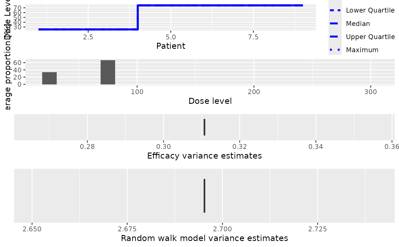
This plot method can be applied to PseudoDualFlexiSimulations objects in
order to summarize them graphically. Possible types of plots at the moment
are:
- trajectory
Summary of the trajectory of the simulated trials
- dosesTried
Average proportions of the doses tested in patients
- sigma2
The variance of the efficacy responses
- sigma2betaW
The variance of the random walk model
You can specify one or both of these in the type argument.
Examples
# Obtain the plot for the simulation results if DLE and efficacy responses
# are considered in the simulations.
emptydata <- DataDual(doseGrid = seq(25, 300, 25))

# The DLE model must be of 'ModelTox' (e.g 'LogisticIndepBeta') class.
dle_model <- LogisticIndepBeta(
  binDLE = c(1.05, 1.8),
  DLEweights = c(3, 3),
  DLEdose = c(25, 300),
  data = emptydata
)

# The efficacy model must be of 'EffFlexi' class.
eff_model <- EffFlexi(
  eff = c(1.223, 2.513),
  eff_dose = c(25, 300),
  sigma2W = c(a = 0.1, b = 0.1),
  sigma2betaW = c(a = 20, b = 50),
  rw1 = FALSE,
  data = emptydata
)

# The escalation rule using the 'NextBestMaxGainSamples' class.
my_next_best <- NextBestMaxGainSamples(
  prob_target_drt = 0.35,
  prob_target_eot = 0.3,
  derive = function(samples) {
    as.numeric(quantile(samples, prob = 0.3))
  },
  mg_derive = function(mg_samples) {
    as.numeric(quantile(mg_samples, prob = 0.5))
  }
)

# The cohort size, size of 3 subjects.
my_size <- CohortSizeConst(size = 3)

# Allow increase of 200%.
my_increments <- IncrementsRelative(intervals = 0, increments = 2)

# Define the stopping rule. Stop when the maximum sample size of 36 patients has
# been reached or when the next dose is NA.
my_stopping <- StoppingMinPatients(nPatients = 36) | StoppingMissingDose()

# Specify the design.
design <- DualResponsesSamplesDesign(
  nextBest = my_next_best,
  cohort_size = my_size,
  startingDose = 25,
  model = dle_model,
  eff_model = eff_model,
  data = emptydata,
  stopping = my_stopping,
  increments = my_increments
)
# Specify the true DLE curve and the true expected efficacy values
# at all dose levels.
my_truth_dle <- probFunction(dle_model, phi1 = -53.66584, phi2 = 10.50499)

my_truth_eff <- c(
  -0.5478867,
  0.1645417,
  0.5248031,
  0.7604467,
  0.9333009,
  1.0687031,
  1.1793942,
  1.2726408,
  1.3529598,
  1.4233411,
  1.4858613,
  1.5420182
)

# The true gain curve.
my_truth_gain <- function(dose) {
  return((myTruthEff(dose)) / (1 + (myTruthDLE(dose) / (1 - myTruthDLE(dose)))))
}

# MCMC options.
my_options <- McmcOptions(burnin = 10, step = 1, samples = 20)

# For illustration purpose only 1 simulation is produced.
my_sim <- simulate(
  object = design,
  args = NULL,
  trueDLE = my_truth_dle,
  trueEff = my_truth_eff,
  trueSigma2 = 0.025,
  trueSigma2betaW = 1,
  mcmcOptions = my_options,
  nsim = 1,
  seed = 819,
  parallel = FALSE
)

# Plot the simulated results.
print(plot(my_sim))
