Plot simulations

Summarize the simulations with plots

Usage

# S4 method for class 'PseudoDualSimulations,missing'
plot(x, y, type = c("trajectory", "dosesTried", "sigma2"), ...)

Arguments

x

the PseudoDualSimulations object we want to plot from

y

missing

type

the type of plots you want to obtain.

...

not used

Value

A single ggplot object if a single plot is asked for, otherwise a gridExtra{gTree} object.

Details

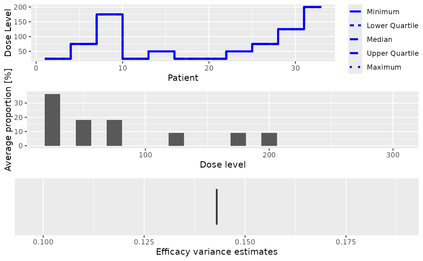
This plot method can be applied to PseudoDualSimulations objects in order to summarize them graphically. Possible types of plots at the moment are:

trajectory

Summary of the trajectory of the simulated trials

dosesTried

Average proportions of the doses tested in patients

sigma2

The variance of the efficacy responses

You can specify one or both of these in the type argument.

Examples

# Obtain the plot for the simulation results if DLE and efficacy responses
# are considered in the simulations.

# Example to run simulations when no samples are used. The data object
# must be defined with doses >= 1:
emptydata <- DataDual(doseGrid = seq(25, 300, 25), placebo = FALSE)

# The DLE model must be of 'ModelTox' (e.g 'LogisticIndepBeta') class.
dle_model <- LogisticIndepBeta(
  binDLE = c(1.05, 1.8),
  DLEweights = c(3, 3),
  DLEdose = c(25, 300),
  data = emptydata
)

# The efficacy model must be of 'ModelEff' (e.g 'Effloglog') class.
eff_model <- Effloglog(
  eff = c(1.223, 2.513), eff_dose = c(25, 300),
  nu = c(a = 1, b = 0.025),
  data = emptydata
)

# The escalation rule using the 'NextBestMaxGain' class.
my_next_best <- NextBestMaxGain(
  prob_target_drt = 0.35,
  prob_target_eot = 0.3
)

# Allow increase of 200%.
my_increments <- IncrementsRelative(intervals = 0, increments = 2)

# Cohort size of 3.
my_size <- CohortSizeConst(size = 3)

# Stop only when 36 subjects are treated or next dose is NA.
my_stopping <- StoppingMinPatients(nPatients = 36) | StoppingMissingDose()

# Now specify the design with all the above information and starting with a
# dose of 25 (for details please refer to the 'DualResponsesDesign' example).
my_design <- DualResponsesDesign(
  nextBest = my_next_best,
  model = dle_model,
  eff_model = eff_model,
  stopping = my_stopping,
  increments = my_increments,
  cohort_size = my_size,
  data = emptydata,
  startingDose = 25
)

# Specify the true DLE and efficacy curves.
my_truth_dle <- probFunction(dle_model, phi1 = -53.66584, phi2 = 10.50499)
my_truth_eff <- efficacyFunction(eff_model, theta1 = -4.818429, theta2 = 3.653058)

# Run simulations (for illustration purpose only 1 simulation is produced).
my_sim <- simulate(
  object = my_design,
  args = NULL,
  trueDLE = my_truth_dle,
  trueEff = my_truth_eff,
  trueNu = 1 / 0.025,
  nsim = 1,
  seed = 819,
  parallel = FALSE
)

# Plot the simulation results.
print(plot(my_sim))

# Example if DLE and efficacy samples are involved.
# The escalation rule using the 'NextBestMaxGainSamples' class.
my_next_best <- NextBestMaxGainSamples(
  prob_target_drt = 0.35,
  prob_target_eot = 0.3,
  derive = function(samples) {
    as.numeric(quantile(samples, prob = 0.3))
  },
  mg_derive = function(mg_samples) {
    as.numeric(quantile(mg_samples, prob = 0.5))
  }
)

# The design of 'DualResponsesSamplesDesign' class.
my_design <- DualResponsesSamplesDesign(
  nextBest = my_next_best,
  cohort_size = my_size,
  startingDose = 25,
  model = dle_model,
  eff_model = eff_model,
  data = emptydata,
  stopping = my_stopping,
  increments = my_increments
)

# Options for MCMC.
my_options <- McmcOptions(burnin = 10, step = 1, samples = 20)

# For illustration purpose only 1 simulation is produced (nsim = 1).
my_sim <- simulate(
  object = my_design,
  args = NULL,
  trueDLE = my_truth_dle,
  trueEff = my_truth_eff,
  trueNu = 1 / 0.025,
  nsim = 1,
  mcmcOptions = my_options,
  seed = 819,
  parallel = FALSE
)

# Plot the simulation results.
print(plot(my_sim))