Plot PseudoDualSimulationsSummary

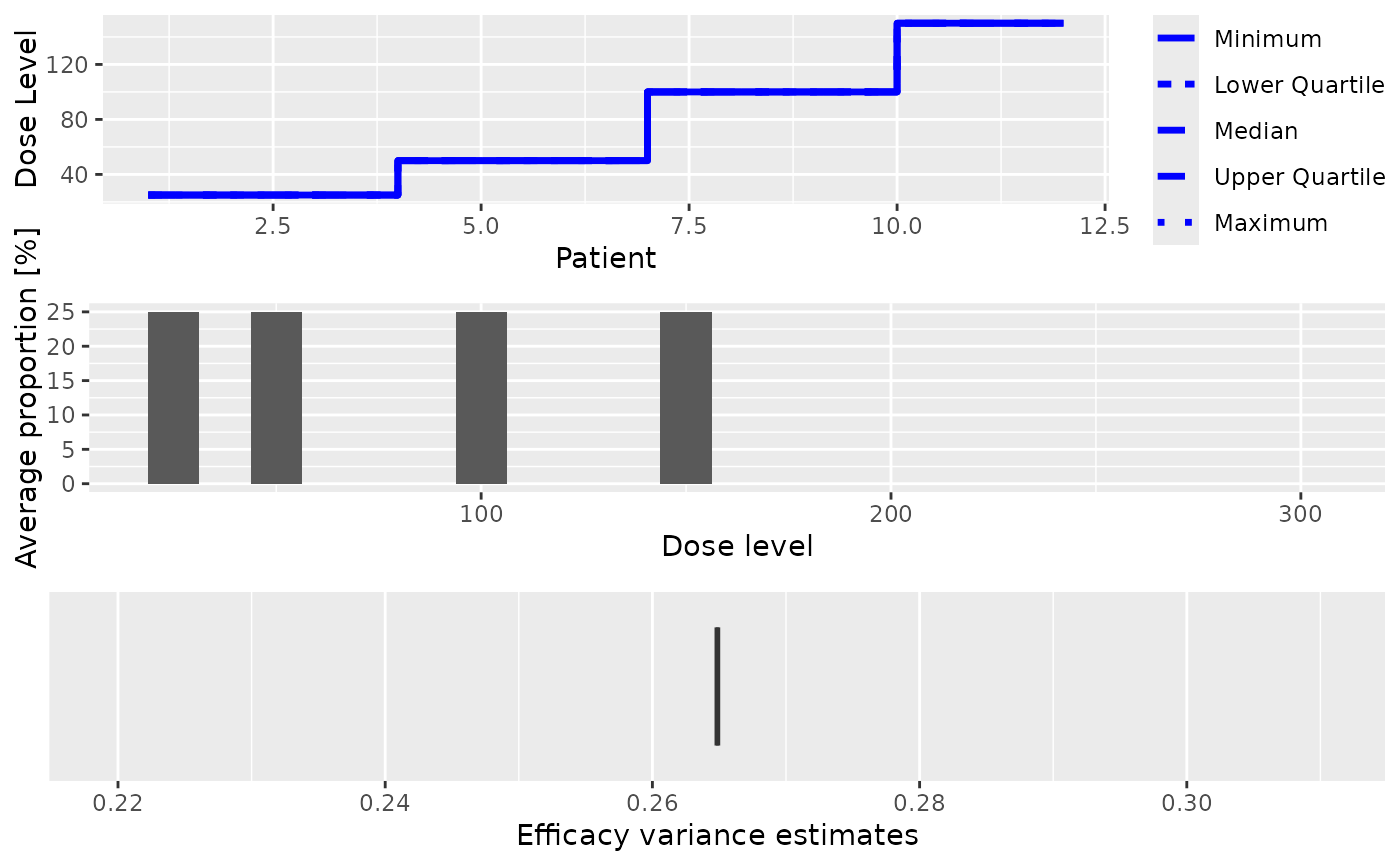
Plot the summary of PseudoDualSimulations.

This plot method can be applied to PseudoDualSimulationsSummary objects in order to summarize them graphically. Possible type of plots at the moment are those listed in plot,PseudoSimulationsSummary,missing-method plus:

meanEffFit

Plot showing the fitted dose-efficacy curve. If no samples are involved, only the average fitted dose-efficacy curve across the trials will be plotted. If samples (DLE and efficacy) are involved, the average fitted dose-efficacy curve across the trials, together with the 95% credibility interval; and comparison with the assumed truth (as specified by the trueEff argument to summary,PseudoDualSimulations-method)

You can specify any subset of these in the type argument.

Usage

# S4 method for class 'PseudoDualSimulationsSummary,missing'
plot(
  x,
  y,
  type = c("nObs", "doseSelected", "propDLE", "nAboveTargetEndOfTrial", "meanFit",
    "meanEffFit"),
  ...
)

Arguments

x

(PseudoDualSimulationsSummary)
the object we want to plot from.

y

(missing)
not used.

type

(character)
the types of plots you want to obtain.

...

not used.

Value

A single ggplot2 object if a single plot is asked for, otherwise a gtable object.

Examples

# Obtain the summary plot for the simulation results if DLE and efficacy
# responses are considered in the simulations.

# In the example when no samples are used a data object with doses >= 1
# needs to be defined.
emptydata <- DataDual(doseGrid = seq(25, 300, 25), placebo = FALSE)

# The DLE model must be of 'ModelTox' (e.g 'LogisticIndepBeta') class.
dle_model <- LogisticIndepBeta(
  binDLE = c(1.05, 1.8),
  DLEweights = c(3, 3),
  DLEdose = c(25, 300),
  data = emptydata
)

# The efficacy model of 'ModelEff' (e.g 'Effloglog') class.
eff_model <- Effloglog(
  eff = c(1.223, 2.513),
  eff_dose = c(25, 300),
  nu = c(a = 1, b = 0.025),
  data = emptydata
)

# The escalation rule using the 'NextBestMaxGain' class.
my_next_best <- NextBestMaxGain(
  prob_target_drt = 0.35,
  prob_target_eot = 0.3
)

# Allow increase of 200%.
my_increments <- IncrementsRelative(intervals = 0, increments = 2)

# Cohort size of 3.
my_size <- CohortSizeConst(size = 3)

# Stop when 10 subjects are treated (for illustration only).
my_stopping <- StoppingMinPatients(nPatients = 10)

## Now specified the design with all the above information and starting with a dose of 25

# Specify the design. (For details please refer to the 'DualResponsesDesign' example.)
my_design <- DualResponsesDesign(
  nextBest = my_next_best,
  model = dle_model,
  eff_model = eff_model,
  stopping = my_stopping,
  increments = my_increments,
  cohort_size = my_size,
  data = emptydata,
  startingDose = 25
)

# Specify the true DLE and efficacy curves.
my_truth_dle <- probFunction(dle_model, phi1 = -53.66584, phi2 = 10.50499)
my_truth_eff <- efficacyFunction(eff_model, theta1 = -4.818429, theta2 = 3.653058)

# \donttest{
# For illustration purpose only 1 simulation is produced.
my_sim <- simulate(
  object = my_design,
  args = NULL,
  trueDLE = my_truth_dle,
  trueEff = my_truth_eff,
  trueNu = 1 / 0.025,
  nsim = 1,
  mcmcOptions = McmcOptions(burnin = 10, step = 1, samples = 50),
  seed = 819,
  parallel = FALSE
)

# Summary of the simulations.
my_sum <- summary(
  my_sim,
  trueDLE = my_truth_dle,
  trueEff = my_truth_eff
)

# Plot the summary of the simulations.
print(plot(my_sum))
# }

# Example where DLE and efficacy samples are involved.
# Please refer to design-method 'simulate DualResponsesSamplesDesign' examples
# for details.
# Specify the next best method.
my_next_best <- NextBestMaxGainSamples(
  prob_target_drt = 0.35,
  prob_target_eot = 0.3,
  derive = function(samples) {
    as.numeric(quantile(samples, prob = 0.3))
  },
  mg_derive = function(mg_samples) {
    as.numeric(quantile(mg_samples, prob = 0.5))
  }
)

# Specify the design.
my_design <- DualResponsesSamplesDesign(
  nextBest = my_next_best,
  cohort_size = my_size,
  startingDose = 25,
  model = dle_model,
  eff_model = eff_model,
  data = emptydata,
  stopping = my_stopping,
  increments = my_increments
)

# MCMC options.
my_options <- McmcOptions(burnin = 10, step = 2, samples = 50)

# \donttest{
# For illustration purpose only 1 simulation is produced.
my_sim <- simulate(
  object = my_design,
  args = NULL,
  trueDLE = my_truth_dle,
  trueEff = my_truth_eff,
  trueNu = 1 / 0.025,
  nsim = 1,
  mcmcOptions = my_options,
  seed = 819,
  parallel = FALSE
)


# Generate a summary of the simulations.
my_sum <- summary(
  my_sim,
  trueDLE = my_truth_dle,
  trueEff = my_truth_eff
)

# Plot the summary of the simulations.
print(plot(my_sum))
# }

# Example where the 'EffFlexi' class is used for the efficacy model.
eff_model <- EffFlexi(
  eff = c(1.223, 2.513),
  eff_dose = c(25, 300),
  sigma2W = c(a = 0.1, b = 0.1),
  sigma2betaW = c(a = 20, b = 50),
  rw1 = FALSE,
  data = emptydata
)

# Specify the design.
my_design <- DualResponsesSamplesDesign(
  nextBest = my_next_best,
  cohort_size = my_size,
  startingDose = 25,
  model = dle_model,
  eff_model = eff_model,
  data = emptydata,
  stopping = my_stopping,
  increments = my_increments
)

# Specify the true DLE curve and the true expected efficacy values at all dose levels.
my_truth_dle <- probFunction(dle_model, phi1 = -53.66584, phi2 = 10.50499)

my_truth_eff <- c(
  -0.5478867, 0.1645417, 0.5248031, 0.7604467,
  0.9333009, 1.0687031, 1.1793942, 1.2726408,
  1.3529598, 1.4233411, 1.4858613, 1.5420182
)

# Define the true gain curve.
my_truth_gain <- function(dose) {
  return((my_truth_eff(dose)) / (1 + (my_truth_dle(dose) / (1 - my_truth_dle(dose)))))
}

# \donttest{
## The simulations
## For illustration purpose only 1 simulation is produced (nsim=1).
mySim <- simulate(
  object = my_design,
  args = NULL,
  trueDLE = my_truth_dle,
  trueEff = my_truth_eff,
  trueSigma2 = 0.025,
  trueSigma2betaW = 1,
  nsim = 1,
  mcmcOptions = my_options,
  seed = 819,
  parallel = FALSE
)

# Produce a summary of the simulations.
my_sum <- summary(
  my_sim,
  trueDLE = my_truth_dle,
  trueEff = my_truth_eff
)

# Plot the summary of the simulations.
print(plot(my_sim))

# }