Plotting dose-toxicity and dose-biomarker model fits

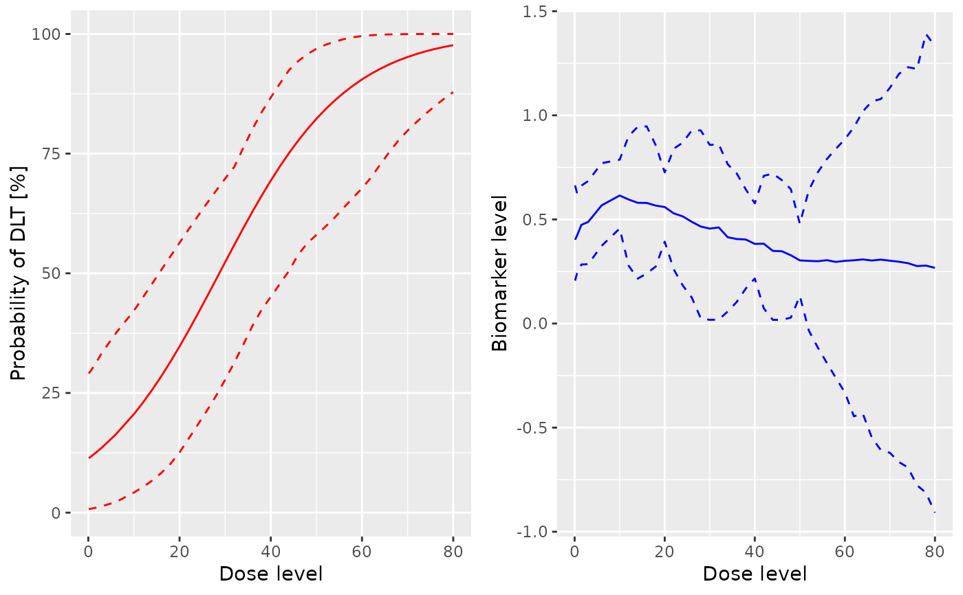
When we have the dual endpoint model, also the dose-biomarker fit is shown in the plot

Usage

# S4 method for Samples,DualEndpoint
plot(x, y, data, extrapolate = TRUE, showLegend = FALSE, ...)

Arguments

x

the Samples object

y

the DualEndpoint object

data

the DataDual object

extrapolate

should the biomarker fit be extrapolated to the whole dose grid? (default)

showLegend

should the legend be shown? (not default)

...

additional arguments for the parent method plot,Samples,GeneralModel-method

Value

This returns the ggplot

object with the dose-toxicity and dose-biomarker model fits

Examples

# nolint start

# Create some data
data <- DataDual(
  x=c(0.1, 0.5, 1.5, 3, 6, 10, 10, 10,
      20, 20, 20, 40, 40, 40, 50, 50, 50),
  y=c(0, 0, 0, 0, 0, 0, 1, 0,
      0, 1, 1, 0, 0, 1, 0, 1, 1),
  w=c(0.31, 0.42, 0.59, 0.45, 0.6, 0.7, 0.55, 0.6,
      0.52, 0.54, 0.56, 0.43, 0.41, 0.39, 0.34, 0.38, 0.21),
  doseGrid=c(0.1, 0.5, 1.5, 3, 6,
             seq(from=10, to=80, by=2)))
#> Used default patient IDs!
#> Used best guess cohort indices!

# Initialize the Dual-Endpoint model (in this case RW1)
model <- DualEndpointRW(mean = c(0, 1),
                        cov = matrix(c(1, 0, 0, 1), nrow=2),
                        sigma2betaW = 0.01,
                        sigma2W = c(a=0.1, b=0.1),
                        rho = c(a=1, b=1),
                        rw1 = TRUE)

# Set-up some MCMC parameters and generate samples from the posterior
options <- McmcOptions(burnin=100,
                       step=2,
                       samples=500)
set.seed(94)
samples <- mcmc(data, model, options)

# Plot the posterior mean  (and empirical 2.5 and 97.5 percentile)
# for the prob(DLT) by doses and the Biomarker by doses
#grid.arrange(plot(x = samples, y = model, data = data))

plot(x = samples, y = model, data = data)


# nolint end