Simulate Method for the DesignGrouped Class

A simulate method for DesignGrouped designs.

Usage

# S4 method for DesignGrouped
simulate(
  object,
  nsim = 1L,
  seed = NULL,
  truth,
  combo_truth,
  args = data.frame(),
  firstSeparate = FALSE,
  mcmcOptions = McmcOptions(),
  parallel = FALSE,
  nCores = min(parallelly::availableCores(), 5),
  ...
)

Arguments

object

(DesignGrouped)
the design we want to simulate trials from.

nsim

(number)
how many trials should be simulated.

seed

(RNGstate)
generated with set_seed().

truth

(function)
a function which takes as input a dose (vector) and returns the true probability (vector) for toxicity for the mono arm. Additional arguments can be supplied in args.

combo_truth

(function)
same as truth but for the combo arm.

args

(data.frame)
optional data.frame with arguments that work for both the truth and combo_truth functions. The column names correspond to the argument names, the rows to the values of the arguments. The rows are appropriately recycled in the nsim simulations.

firstSeparate

(flag)
whether to enroll the first patient separately from the rest of the cohort and close the cohort in case a DLT occurs in this first patient.

mcmcOptions

(McmcOptions)
MCMC options for each evaluation in the trial.

parallel

(flag)
whether the simulation runs are parallelized across the cores of the computer.

nCores

(number)
how many cores should be used for parallel computing.

...

not used.

Value

A list of mono and combo simulation results as Simulations objects.

Examples

# Assemble ingredients for our group design.
my_stopping <- StoppingTargetProb(target = c(0.2, 0.35), prob = 0.5) |
  StoppingMinPatients(10) |
  StoppingMissingDose()
my_increments <- IncrementsDoseLevels(levels = 3L)
my_next_best <- NextBestNCRM(
  target = c(0.2, 0.3),
  overdose = c(0.3, 1),
  max_overdose_prob = 0.3
)
my_cohort_size <- CohortSizeConst(3)
empty_data <- Data(doseGrid = c(0.1, 0.5, 1.5, 3, 6, seq(from = 10, to = 80, by = 2)))
my_model <- LogisticLogNormalGrouped(
  mean = c(-4, -4, -4, -4),
  cov = diag(rep(6, 4)),
  ref_dose = 0.1
)

# Put together the design. Note that if we only specify the mono arm,
# then the combo arm is having the same settings.
my_design <- DesignGrouped(
  model = my_model,
  mono = Design(
    model = my_model,
    stopping = my_stopping,
    increments = my_increments,
    nextBest = my_next_best,
    cohort_size = my_cohort_size,
    data = empty_data,
    startingDose = 0.1
  ),
  first_cohort_mono_only = TRUE,
  same_dose_for_all = TRUE
)

# Set up a realistic simulation scenario.
my_truth <- function(x) plogis(-4 + 0.2 * log(x / 0.1))
my_combo_truth <- function(x) plogis(-4 + 0.5 * log(x / 0.1))
matplot(
  x = empty_data@doseGrid,
  y = cbind(
    mono = my_truth(empty_data@doseGrid),
    combo = my_combo_truth(empty_data@doseGrid)
  ),
  type = "l",
  ylab = "true DLT prob",
  xlab = "dose"
)
legend("topright", c("mono", "combo"), lty = c(1, 2), col = c(1, 2))

# Start the simulations.
set.seed(123)
my_sims <- simulate(
  my_design,
  nsim = 1, # This should be at least 100 in actual applications.
  seed = 123,
  truth = my_truth,
  combo_truth = my_combo_truth
)

# Looking at the summary of the simulations:
mono_sims_sum <- summary(my_sims$mono, truth = my_truth)
combo_sims_sum <- summary(my_sims$combo, truth = my_combo_truth)

mono_sims_sum
#> Summary of 1 simulations
#> 
#> Target toxicity interval was 20, 35 %
#> Target dose interval corresponding to this was NA, NA 
#> Intervals are corresponding to 10 and 90 % quantiles
#> 
#> Number of patients overall : mean 12 (12, 12) 
#> Number of patients treated above target tox interval : mean 0 (0, 0) 
#> Proportions of DLTs in the trials : mean 0 % (0 %, 0 %) 
#> Mean toxicity risks for the patients on active : mean 3 % (3 %, 3 %) 
#> Doses selected as MTD : mean 14 (14, 14) 
#> True toxicity at doses selected : mean 5 % (5 %, 5 %) 
#> Proportion of trials selecting target MTD: 0 %
#> Dose most often selected as MTD: 14 
#> Observed toxicity rate at dose most often selected: NaN %
#> Fitted toxicity rate at dose most often selected : mean 7 % (7 %, 7 %) 
#> Stop reason triggered:
#>  P(0.2 ≤ prob(DLE | NBD) ≤ 0.35) ≥ 0.5 :  0 %
#>  ≥ 10 patients dosed :  100 %
#>  Stopped because of missing dose :  0 %
combo_sims_sum
#> Summary of 1 simulations
#> 
#> Target toxicity interval was 20, 35 %
#> Target dose interval corresponding to this was 18.6, NA 
#> Intervals are corresponding to 10 and 90 % quantiles
#> 
#> Number of patients overall : mean 12 (12, 12) 
#> Number of patients treated above target tox interval : mean 0 (0, 0) 
#> Proportions of DLTs in the trials : mean 17 % (17 %, 17 %) 
#> Mean toxicity risks for the patients on active : mean 10 % (10 %, 10 %) 
#> Doses selected as MTD : mean 12 (12, 12) 
#> True toxicity at doses selected : mean 17 % (17 %, 17 %) 
#> Proportion of trials selecting target MTD: 0 %
#> Dose most often selected as MTD: 12 
#> Observed toxicity rate at dose most often selected: NaN %
#> Fitted toxicity rate at dose most often selected : mean 16 % (16 %, 16 %) 
#> Stop reason triggered:
#>  P(0.2 ≤ prob(DLE | NBD) ≤ 0.35) ≥ 0.5 :  0 %
#>  ≥ 10 patients dosed :  100 %
#>  Stopped because of missing dose :  0 %

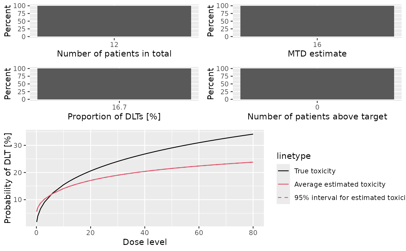
plot(mono_sims_sum)
plot(combo_sims_sum)


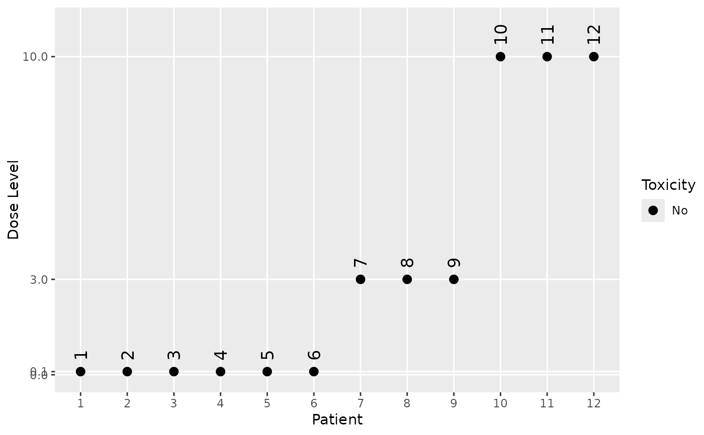
# Looking at specific simulated trials:
trial_index <- 1
plot(my_sims$mono@data[[trial_index]])

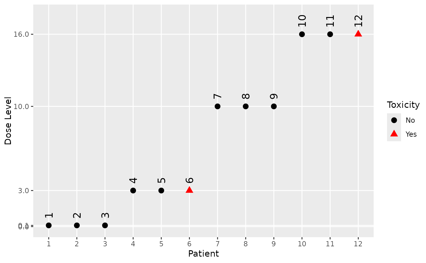
plot(my_sims$combo@data[[trial_index]])