Plot dual-endpoint simulations

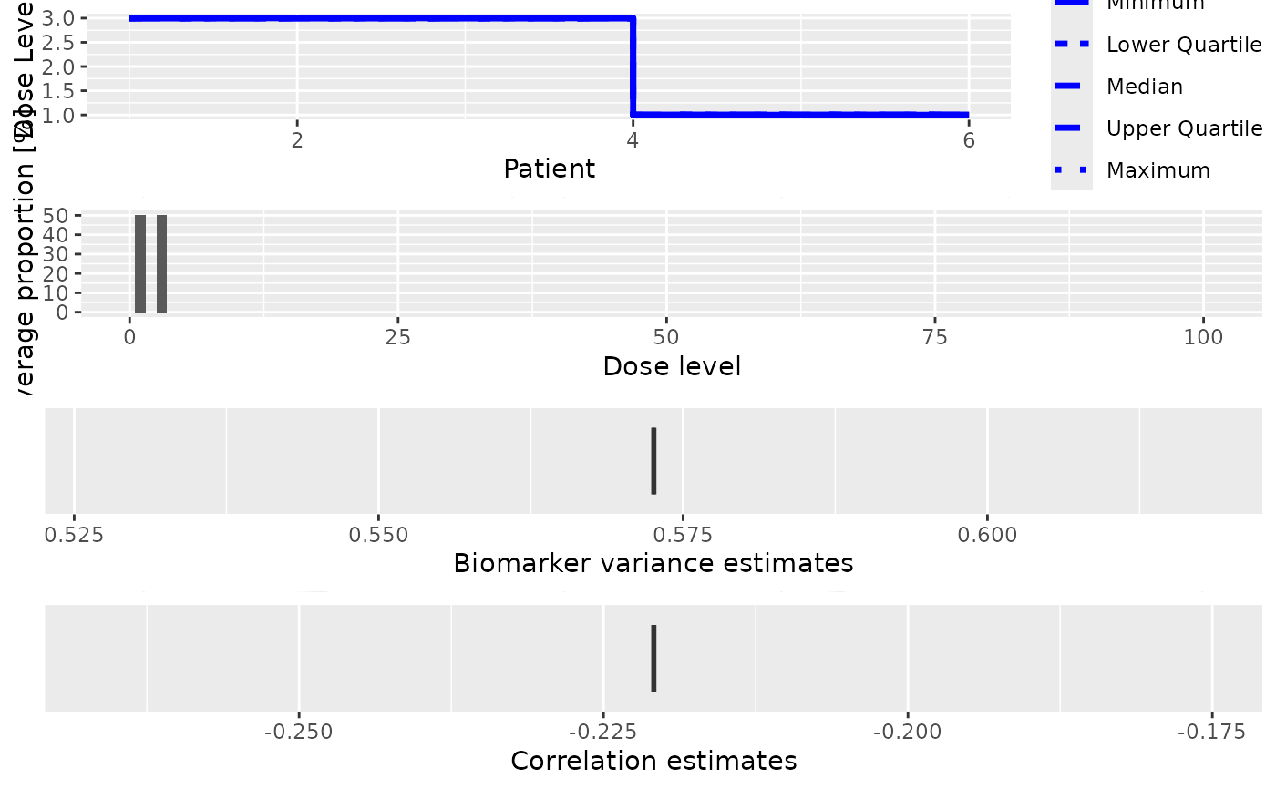
This plot method can be applied to DualSimulations objects in order to summarize them graphically. In addition to the standard plot types, there is

sigma2W

Plot a boxplot of the final biomarker variance estimates in the simulated trials

rho

Plot a boxplot of the final correlation estimates in the simulated trials

Usage

# S4 method for class 'DualSimulations,missing'
plot(x, y, type = c("trajectory", "dosesTried", "sigma2W", "rho"), ...)

Arguments

x

the DualSimulations object we want to plot from

y

missing

type

the type of plots you want to obtain.

...

not used

Value

A single ggplot object if a single plot is asked for, otherwise a gtable object.

Examples

# Define the dose-grid.
emptydata <- DataDual(doseGrid = c(1, 3, 5, 10, 15, 20, 25, 40, 50, 80, 100))

# Create some data.
my_data <- DataDual(
  x = c(
    0.1,
    0.5,
    1.5,
    3,
    6,
    10,
    10,
    10,
    20,
    20,
    20,
    40,
    40,
    40,
    50,
    50,
    50
  ),
  y = c(
    0,
    0,
    0,
    0,
    0,
    0,
    1,
    0,
    0,
    1,
    1,
    0,
    0,
    1,
    0,
    1,
    1
  ),
  ID = 1:17,
  cohort = c(
    1L,
    2L,
    3L,
    4L,
    5L,
    6L,
    6L,
    6L,
    7L,
    7L,
    7L,
    8L,
    8L,
    8L,
    9L,
    9L,
    9L
  ),
  w = c(
    0.31,
    0.42,
    0.59,
    0.45,
    0.6,
    0.7,
    0.55,
    0.6,
    0.52,
    0.54,
    0.56,
    0.43,
    0.41,
    0.39,
    0.34,
    0.38,
    0.21
  ),
  doseGrid = c(
    0.1,
    0.5,
    1.5,
    3,
    6,
    seq(from = 10, to = 80, by = 2)
  )
)

# Initialize the CRM model.
my_model <- DualEndpointRW(
  mean = c(0, 1),
  cov = matrix(c(1, 0, 0, 1), nrow = 2),
  sigma2betaW = 0.01,
  sigma2W = c(a = 0.1, b = 0.1),
  rho = c(a = 1, b = 1),
  rw1 = TRUE
)

# Choose the rule for selecting the next dose.
my_next_best <- NextBestDualEndpoint(
  target = c(0.9, 1),
  overdose = c(0.35, 1),
  max_overdose_prob = 0.25
)

# Choose the rule for the cohort-size
mySize1 <- CohortSizeRange(
  intervals = c(0, 30),
  cohort_size = c(1, 3)
)
mySize2 <- CohortSizeDLT(
  intervals = c(0, 1),
  cohort_size = c(1, 3)
)
mySize <- maxSize(mySize1, mySize2)

# Choose the rule for stopping
myStopping4 <- StoppingTargetBiomarker(
  target = c(0.9, 1),
  prob = 0.5
)
myStopping <- myStopping4 | StoppingMinPatients(40)

my_size1 <- CohortSizeRange(
  intervals = c(0, 30),
  cohort_size = c(1, 3)
)
my_size2 <- CohortSizeDLT(
  intervals = c(0, 1),
  cohort_size = c(1, 3)
)
my_size <- maxSize(my_size1, my_size2)

# Choose the rule for stopping
my_stopping4 <- StoppingTargetBiomarker(
  target = c(0.9, 1),
  prob = 0.5
)
my_stopping <- my_stopping4 | StoppingMinPatients(40) | StoppingMissingDose()

# Choose the rule for dose increments
my_increments <- IncrementsRelative(
  intervals = c(0, 20),
  increments = c(1, 0.33)
)

# Initialize the design

my_design <- DualDesign(
  model = my_model,
  data = emptydata,
  nextBest = my_next_best,
  stopping = my_stopping,
  increments = my_increments,
  cohort_size = CohortSizeConst(3),
  startingDose = 3
)

# Define scenarios for the TRUE toxicity and efficacy profiles.
beta_mod <- function(dose, e0, eMax, delta1, delta2, scal) {
  maxDens <- (delta1^delta1) *
    (delta2^delta2) /
    ((delta1 + delta2)^(delta1 + delta2))
  dose <- dose / scal
  e0 + eMax / maxDens * (dose^delta1) * (1 - dose)^delta2
}

true_biomarker <- function(dose) {
  beta_mod(
    dose,
    e0 = 0.2,
    eMax = 0.6,
    delta1 = 5,
    delta2 = 5 * 0.5 / 0.5,
    scal = 100
  )
}

true_tox <- function(dose) {
  pnorm((dose - 60) / 10)
}

# Draw the TRUE profiles
par(mfrow = c(1, 2))
curve(true_tox(x), from = 0, to = 80)
curve(true_biomarker(x), from = 0, to = 80)

# Run the simulation on the desired design.
# We only generate 1 trial outcome here for illustration, for the actual study.
# Also for illustration purpose, we will use 5 burn-ins to generate 20 samples,
# this should be increased of course.
my_sims <- simulate(
  object = my_design,
  trueTox = true_tox,
  trueBiomarker = true_biomarker,
  sigma2W = 0.01,
  rho = 0,
  nsim = 1,
  parallel = FALSE,
  seed = 9,
  startingDose = 6,
  mcmcOptions = McmcOptions(
    burnin = 1,
    step = 1,
    samples = 2
  )
)

# Plot the results of the simulation.
print(plot(my_sims))
#> Warning: Using `size` aesthetic for lines was deprecated in ggplot2 3.4.0.
#> ℹ Please use `linewidth` instead.
#> ℹ The deprecated feature was likely used in the crmPack package.
#>   Please report the issue at <https://github.com/openpharma/crmPack/issues>.
#> Warning: `qplot()` was deprecated in ggplot2 3.4.0.
#> ℹ The deprecated feature was likely used in the crmPack package.
#>   Please report the issue at <https://github.com/openpharma/crmPack/issues>.