Plot Model-Based Design Simulation Summary

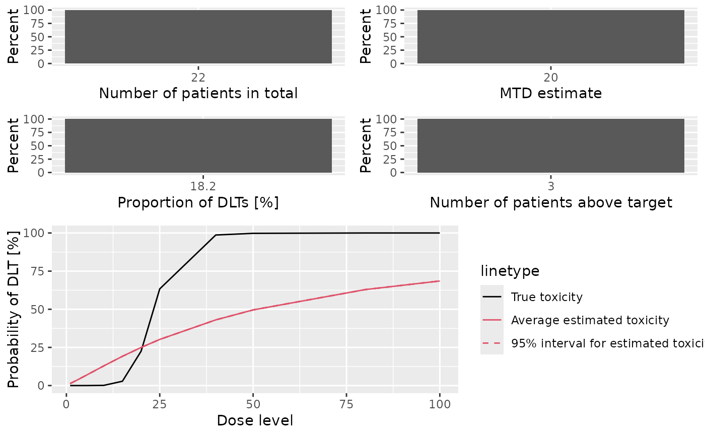
Graphical display of the simulation summary.

This plot method can be applied to SimulationsSummary objects in order to summarize them graphically. Possible type of plots at the moment are those listed in plot,GeneralSimulationsSummary,missing-method plus:

meanFit

Plot showing the average fitted dose-toxicity curve across the trials, together with 95% credible intervals, and comparison with the assumed truth (as specified by the truth argument to summary,Simulations-method)

You can specify any subset of these in the type argument.

Usage

# S4 method for class 'SimulationsSummary,missing'
plot(
  x,
  y,
  type = c("nObs", "doseSelected", "propDLTs", "nAboveTarget", "meanFit"),
  ...
)

Arguments

x

(SimulationsSummary)
the object we want to plot from.

y

(missing)
not used.

type

(character)
the types of plots you want to obtain.

...

not used.

Value

A single ggplot object if a single plot is asked for, otherwise a gtable object.

Examples

# nolint start

# Define the dose-grid
emptydata <- Data(doseGrid = c(1, 3, 5, 10, 15, 20, 25, 40, 50, 80, 100))

# Initialize the CRM model
model <- LogisticLogNormal(
  mean = c(-0.85, 1),
  cov = matrix(c(1, -0.5, -0.5, 1), nrow = 2),
  ref_dose = 56
)

# Choose the rule for selecting the next dose
myNextBest <- NextBestNCRM(
  target = c(0.2, 0.35),
  overdose = c(0.35, 1),
  max_overdose_prob = 0.25
)

# Choose the rule for the cohort-size
mySize1 <- CohortSizeRange(
  intervals = c(0, 30),
  cohort_size = c(1, 3)
)
mySize2 <- CohortSizeDLT(
  intervals = c(0, 1),
  cohort_size = c(1, 3)
)
mySize <- maxSize(mySize1, mySize2)

# Choose the rule for stopping
myStopping1 <- StoppingMinCohorts(nCohorts = 3)
myStopping2 <- StoppingTargetProb(
  target = c(0.2, 0.35),
  prob = 0.5
)
myStopping3 <- StoppingMinPatients(nPatients = 20)
myStopping <- (myStopping1 & myStopping2) | myStopping3

# Choose the rule for dose increments
myIncrements <- IncrementsRelative(
  intervals = c(0, 20),
  increments = c(1, 0.33)
)

# Initialize the design
design <- Design(
  model = model,
  nextBest = myNextBest,
  stopping = myStopping,
  increments = myIncrements,
  cohort_size = mySize,
  data = emptydata,
  startingDose = 3
)

## define the true function
myTruth <- probFunction(model, alpha0 = 7, alpha1 = 8)

# Run the simulation on the desired design
# We only generate 1 trial outcomes here for illustration, for the actual study
# this should be increased of course
options <- McmcOptions(
  burnin = 10,
  step = 1,
  samples = 100
)
time <- system.time(
  mySims <- simulate(
    design,
    args = NULL,
    truth = myTruth,
    nsim = 1,
    seed = 819,
    mcmcOptions = options,
    parallel = FALSE
  )
)[3]

# Plot the Summary of the Simulations
plot(summary(mySims, truth = myTruth))


# nolint end