A function that computes the recommended next best dose based on the
corresponding rule nextBest, the posterior samples from the model and
the underlying data.
Usage
nextBest(nextBest, doselimit, samples, model, data, ...)

# S4 method for class 'NextBestEWOC,numeric,Samples,GeneralModel,Data'
nextBest(nextBest, doselimit = Inf, samples, model, data, ...)

# S4 method for class 'NextBestMTD,numeric,Samples,GeneralModel,Data'
nextBest(nextBest, doselimit = Inf, samples, model, data, ...)

# S4 method for class 'NextBestNCRM,numeric,Samples,GeneralModel,Data'
nextBest(nextBest, doselimit = Inf, samples, model, data, ...)

# S4 method for class 'NextBestNCRM,numeric,Samples,GeneralModel,DataParts'
nextBest(nextBest, doselimit = Inf, samples, model, data, ...)

# S4 method for class 'NextBestNCRMLoss,numeric,Samples,GeneralModel,Data'
nextBest(nextBest, doselimit = Inf, samples, model, data, ...)

# S4 method for class 'NextBestThreePlusThree,missing,missing,missing,Data'
nextBest(nextBest, doselimit, samples, model, data, ...)

# S4 method for class 'NextBestDualEndpoint,numeric,Samples,DualEndpoint,Data'
nextBest(nextBest, doselimit = Inf, samples, model, data, ...)

# S4 method for class 'NextBestMinDist,numeric,Samples,GeneralModel,Data'
nextBest(nextBest, doselimit = Inf, samples, model, data, ...)

# S4 method for class 'NextBestInfTheory,numeric,Samples,GeneralModel,Data'
nextBest(nextBest, doselimit = Inf, samples, model, data, ...)

# S4 method for class 'NextBestTD,numeric,missing,LogisticIndepBeta,Data'
nextBest(nextBest, doselimit = Inf, model, data, in_sim = FALSE, ...)

# S4 method for class 'NextBestTDsamples,numeric,Samples,LogisticIndepBeta,Data'
nextBest(nextBest, doselimit = Inf, samples, model, data, in_sim, ...)

# S4 method for class 'NextBestMaxGain,numeric,missing,ModelTox,DataDual'
nextBest(
  nextBest,
  doselimit = Inf,
  model,
  data,
  model_eff,
  in_sim = FALSE,
  ...
)

# S4 method for class 'NextBestMaxGainSamples,numeric,Samples,ModelTox,DataDual'
nextBest(
  nextBest,
  doselimit = Inf,
  samples,
  model,
  data,
  model_eff,
  samples_eff,
  in_sim = FALSE,
  ...
)

# S4 method for class 'NextBestProbMTDLTE,numeric,Samples,GeneralModel,Data'
nextBest(nextBest, doselimit, samples, model, data, ...)

# S4 method for class 'NextBestProbMTDMinDist,numeric,Samples,GeneralModel,Data'
nextBest(nextBest, doselimit, samples, model, data, ...)

# S4 method for class 'NextBestOrdinal,numeric,Samples,GeneralModel,Data'
nextBest(nextBest, doselimit = Inf, samples, model, data, ...)

# S4 method for class 'NextBestOrdinal,numeric,Samples,LogisticLogNormalOrdinal,DataOrdinal'
nextBest(nextBest, doselimit = Inf, samples, model, data, ...)
Arguments
- nextBest
(
NextBest)
the rule for the next best dose.- doselimit
(
number)
the maximum allowed next dose. If it is an infinity (default), then essentially no dose limit will be applied in the course of dose recommendation calculation.- samples
(
Samples)
posterior samples frommodelparameters givendata.- model
(
ModelTox)
the DLT model.- data
(
Data)
data that was used to generate the samples.- ...
additional arguments without method dispatch.
- in_sim
(
flag)
is this method used in simulations? Default asFALSE. If this flag isTRUEand target dose estimates (during trial and end-of-trial) are outside of the dose grid range, the information message is printed by this method.- model_eff
(
EffloglogorEffFlexi)
the efficacy model.- samples_eff
(
Samples)
posterior samples frommodel_effparameters givendata.
Value
A list with the next best dose recommendation (element named value)
from the grid defined in data, and a plot depicting this recommendation
(element named plot). In case of multiple plots also an element
named singlePlots is included. The singlePlots is itself a list with
single plots. An additional list with elements describing the outcome
of the rule can be contained too.
Functions
nextBest(
  nextBest = NextBestEWOC,
  doselimit = numeric,
  samples = Samples,
  model = GeneralModel,
  data = Data
)
: find the next best dose based on the EWOC rule.nextBest( nextBest = NextBestMTD, doselimit = numeric, samples = Samples, model = GeneralModel, data = Data ): find the next best dose based on the MTD rule.nextBest( nextBest = NextBestNCRM, doselimit = numeric, samples = Samples, model = GeneralModel, data = Data ): find the next best dose based on the NCRM method. The additional elementprobsin the output's list contains the target and overdosing probabilities (across all doses in the dose grid) used in the derivation of the next best dose.nextBest( nextBest = NextBestNCRM, doselimit = numeric, samples = Samples, model = GeneralModel, data = DataParts ): find the next best dose based on the NCRM method when two parts trial is used.nextBest( nextBest = NextBestNCRMLoss, doselimit = numeric, samples = Samples, model = GeneralModel, data = Data ): find the next best dose based on the NCRM method and loss function.nextBest( nextBest = NextBestThreePlusThree, doselimit = missing, samples = missing, model = missing, data = Data ): find the next best dose based on the 3+3 method.nextBest( nextBest = NextBestDualEndpoint, doselimit = numeric, samples = Samples, model = DualEndpoint, data = Data ): find the next best dose based on the dual endpoint model. The additional list elementprobscontains the target and overdosing probabilities (across all doses in the dose grid) used in the derivation of the next best dose.nextBest( nextBest = NextBestMinDist, doselimit = numeric, samples = Samples, model = GeneralModel, data = Data ): gives the dose which is below the dose limit and has an estimated DLT probability which is closest to the target dose.nextBest( nextBest = NextBestInfTheory, doselimit = numeric, samples = Samples, model = GeneralModel, data = Data ): gives the appropriate dose within an information theoretic framework.nextBest( nextBest = NextBestTD, doselimit = numeric, samples = missing, model = LogisticIndepBeta, data = Data ): find the next best dose based only on the DLT responses and forLogisticIndepBetamodel class object without DLT samples.nextBest( nextBest = NextBestTDsamples, doselimit = numeric, samples = Samples, model = LogisticIndepBeta, data = Data ): find the next best dose based only on the DLT responses and forLogisticIndepBetamodel class object involving DLT samples.nextBest( nextBest = NextBestMaxGain, doselimit = numeric, samples = missing, model = ModelTox, data = DataDual ): find the next best dose based only on pseudo DLT modelModelToxandEffloglogefficacy model without samples.nextBest( nextBest = NextBestMaxGainSamples, doselimit = numeric, samples = Samples, model = ModelTox, data = DataDual ): find the next best dose based on DLT and efficacy responses with DLT and efficacy samples.nextBest( nextBest = NextBestProbMTDLTE, doselimit = numeric, samples = Samples, model = GeneralModel, data = Data ): find the next best dose based with the highest probability of having a toxicity rate less or equal to the target toxicity level.nextBest( nextBest = NextBestProbMTDMinDist, doselimit = numeric, samples = Samples, model = GeneralModel, data = Data ): find the next best dose based with the highest probability of having a toxicity rate with minimum distance to the target toxicity level.nextBest( nextBest = NextBestOrdinal, doselimit = numeric, samples = Samples, model = GeneralModel, data = Data ): find the next best dose for ordinal CRM models.nextBest( nextBest = NextBestOrdinal, doselimit = numeric, samples = Samples, model = LogisticLogNormalOrdinal, data = DataOrdinal ): find the next best dose for ordinal CRM models.
Examples
# Example of usage for `NextBestEWOC` NextBest class.
# Create the data.
my_data <- Data(
x = c(0.1, 0.5, 1.5, 3, 6, 10, 10, 10),
y = c(0, 0, 0, 0, 0, 0, 1, 0),
ID = 1:8,
cohort = c(0, 1, 2, 3, 4, 5, 5, 5),
doseGrid = c(0.1, 0.5, 1.5, 3, 6, seq(from = 10, to = 80, by = 2))
)
# Initialize the CRM model used to model the data.
my_model <- LogisticLogNormal(
mean = c(-0.85, 1),
cov = matrix(c(1, -0.5, -0.5, 1), nrow = 2),
ref_dose = 56
)
# Set-up some MCMC parameters and generate samples from the posterior.
my_options <- McmcOptions(burnin = 5, step = 1, samples = 10)
my_samples <- mcmc(my_data, my_model, my_options)
# Define the rule for dose increments and calculate the maximum dose allowed.
my_increments <- IncrementsRelative(
intervals = c(0, 20),
increments = c(1, 0.33)
)
next_max_dose <- maxDose(my_increments, data = my_data)
# Define the rule which will be used to select the next best dose
# based on the 'NextBestEWOC' class.
ewoc_next_best <- NextBestEWOC(
target = 0.30,
overdose = c(0.35, 1),
max_overdose_prob = 0.25
)
# Calculate the next best dose.
dose_recommendation <- nextBest(
nextBest = ewoc_next_best,
doselimit = next_max_dose,
samples = my_samples,
model = my_model,
data = my_data
)
# See the probabilities.
dose_recommendation$probs
#> dose overdose
#> [1,] 0.1 0
#> [2,] 0.5 0
#> [3,] 1.5 0
#> [4,] 3.0 0
#> [5,] 6.0 0
#> [6,] 10.0 0
#> [7,] 12.0 0
#> [8,] 14.0 0
#> [9,] 16.0 0
#> [10,] 18.0 0
#> [11,] 20.0 0
#> [12,] 22.0 0
#> [13,] 24.0 0
#> [14,] 26.0 1
#> [15,] 28.0 1
#> [16,] 30.0 1
#> [17,] 32.0 1
#> [18,] 34.0 1
#> [19,] 36.0 1
#> [20,] 38.0 1
#> [21,] 40.0 1
#> [22,] 42.0 1
#> [23,] 44.0 1
#> [24,] 46.0 1
#> [25,] 48.0 1
#> [26,] 50.0 1
#> [27,] 52.0 1
#> [28,] 54.0 1
#> [29,] 56.0 1
#> [30,] 58.0 1
#> [31,] 60.0 1
#> [32,] 62.0 1
#> [33,] 64.0 1
#> [34,] 66.0 1
#> [35,] 68.0 1
#> [36,] 70.0 1
#> [37,] 72.0 1
#> [38,] 74.0 1
#> [39,] 76.0 1
#> [40,] 78.0 1
#> [41,] 80.0 1
# Example of usage for `NextBestMTD` NextBest class.
# Create the data.
my_data <- Data(
x = c(0.1, 0.5, 1.5, 3, 6, 10, 10, 10),
y = c(0, 0, 0, 0, 0, 0, 1, 0),
ID = 1:8,
cohort = c(0, 1, 2, 3, 4, 5, 5, 5),
doseGrid = c(0.1, 0.5, 1.5, 3, 6, seq(from = 10, to = 80, by = 2))
)
# Initialize the CRM model used to model the data.
my_model <- LogisticLogNormal(
mean = c(-0.85, 1),
cov = matrix(c(1, -0.5, -0.5, 1), nrow = 2),
ref_dose = 56
)
# Set-up some MCMC parameters and generate samples from the posterior.
my_options <- McmcOptions(burnin = 5, step = 1, samples = 10)
my_samples <- mcmc(my_data, my_model, my_options)
# Define the rule for dose increments and calculate the maximum dose allowed.
my_increments <- IncrementsRelative(
intervals = c(0, 20),
increments = c(1, 0.33)
)
next_max_dose <- maxDose(my_increments, data = my_data)
# Define the rule which will be used to select the next best dose
# based on the 'NextBestMTD' class.
mtd_next_best <- NextBestMTD(
target = 0.33,
derive = function(mtd_samples) {
quantile(mtd_samples, probs = 0.25)
}
)
# Calculate the next best dose.
dose_recommendation <- nextBest(
nextBest = mtd_next_best,
doselimit = next_max_dose,
samples = my_samples,
model = my_model,
data = my_data
)
# Example of usage for `NextBestNCRM` NextBest class.
# Create the data.
my_data <- Data(
x = c(0.1, 0.5, 1.5, 3, 6, 10, 10, 10),
y = c(0, 0, 0, 0, 0, 0, 1, 0),
ID = 1:8,
cohort = c(0, 1, 2, 3, 4, 5, 5, 5),
doseGrid = c(0.1, 0.5, 1.5, 3, 6, seq(from = 10, to = 80, by = 2))
)
# Initialize the CRM model used to model the data.
my_model <- LogisticLogNormal(
mean = c(-0.85, 1),
cov = matrix(c(1, -0.5, -0.5, 1), nrow = 2),
ref_dose = 56
)
# Set-up some MCMC parameters and generate samples from the posterior.
my_options <- McmcOptions(burnin = 5, step = 1, samples = 10)
my_samples <- mcmc(my_data, my_model, my_options)
# Define the rule for dose increments and calculate the maximum dose allowed.
my_increments <- IncrementsRelative(
intervals = c(0, 20),
increments = c(1, 0.33)
)
next_max_dose <- maxDose(my_increments, data = my_data)
# Define the rule which will be used to select the next best dose
# based on the 'NextBestNCRM' class.
nrcm_next_best <- NextBestNCRM(
target = c(0.2, 0.35),
overdose = c(0.35, 1),
max_overdose_prob = 0.25
)
# Calculate the next best dose.
dose_recommendation <- nextBest(
nextBest = nrcm_next_best,
doselimit = next_max_dose,
samples = my_samples,
model = my_model,
data = my_data
)
# See the probabilities.
dose_recommendation$probs
#> dose target overdose
#> [1,] 0.1 0.0 0.0
#> [2,] 0.5 0.0 0.0
#> [3,] 1.5 0.0 0.0
#> [4,] 3.0 0.0 0.0
#> [5,] 6.0 0.0 0.0
#> [6,] 10.0 0.0 0.0
#> [7,] 12.0 0.0 0.0
#> [8,] 14.0 0.0 0.0
#> [9,] 16.0 0.0 0.0
#> [10,] 18.0 0.0 0.0
#> [11,] 20.0 0.0 0.0
#> [12,] 22.0 0.0 0.0
#> [13,] 24.0 0.0 0.0
#> [14,] 26.0 0.0 0.0
#> [15,] 28.0 0.0 0.0
#> [16,] 30.0 0.1 0.0
#> [17,] 32.0 0.1 0.0
#> [18,] 34.0 0.1 0.0
#> [19,] 36.0 0.4 0.0
#> [20,] 38.0 0.6 0.0
#> [21,] 40.0 0.6 0.0
#> [22,] 42.0 0.6 0.0
#> [23,] 44.0 0.9 0.1
#> [24,] 46.0 0.9 0.1
#> [25,] 48.0 0.9 0.1
#> [26,] 50.0 0.9 0.1
#> [27,] 52.0 0.9 0.1
#> [28,] 54.0 0.9 0.1
#> [29,] 56.0 0.6 0.4
#> [30,] 58.0 0.6 0.4
#> [31,] 60.0 0.6 0.4
#> [32,] 62.0 0.6 0.4
#> [33,] 64.0 0.6 0.4
#> [34,] 66.0 0.6 0.4
#> [35,] 68.0 0.4 0.6
#> [36,] 70.0 0.4 0.6
#> [37,] 72.0 0.4 0.6
#> [38,] 74.0 0.4 0.6
#> [39,] 76.0 0.4 0.6
#> [40,] 78.0 0.4 0.6
#> [41,] 80.0 0.4 0.6
# Example of usage for `NextBestNCRM-DataParts` NextBest class.
# Create the data.
my_data <- DataParts(
x = c(0.1, 0.5, 1.5),
y = c(0, 0, 0),
ID = 1:3,
cohort = 1:3,
doseGrid = c(0.1, 0.5, 1.5, 3, 6, seq(from = 10, to = 80, by = 2)),
part = c(1L, 1L, 1L),
nextPart = 1L,
part1Ladder = c(0.1, 0.5, 1.5, 3, 6, 10)
)
# Initialize the CRM model used to model the data.
my_model <- LogisticLogNormal(
mean = c(-0.85, 1),
cov = matrix(c(1, -0.5, -0.5, 1), nrow = 2),
ref_dose = 56
)
# Set-up some MCMC parameters and generate samples from the posterior.
my_options <- McmcOptions(burnin = 5, step = 1, samples = 10)
my_samples <- mcmc(my_data, my_model, my_options)
# Define the rule for dose increments and calculate the maximum dose allowed.
my_increments <- IncrementsRelativeParts(
dlt_start = 0,
clean_start = 1
)
next_max_dose <- maxDose(my_increments, data = my_data)
# Define the rule which will be used to select the next best dose
# based on the 'NextBestNCRM' class.
nrcm_next_best <- NextBestNCRM(
target = c(0.2, 0.35),
overdose = c(0.35, 1),
max_overdose_prob = 0.25
)
# Calculate the next best dose.
dose_recommendation <- nextBest(
nextBest = nrcm_next_best,
doselimit = next_max_dose,
samples = my_samples,
model = my_model,
data = my_data
)
dose_recommendation
#> $value
#> [1] 3
#>
#> $plot
#> NULL
#>
# Example of usage for `NextBestNCRMLoss` NextBest class.
# Create the data.
my_data <- Data(
x = c(0.1, 0.5, 1.5, 3, 6, 10, 10, 10),
y = c(0, 0, 0, 0, 0, 0, 1, 0),
ID = 1:8,
cohort = c(0, 1, 2, 3, 4, 5, 5, 5),
doseGrid = c(0.1, 0.5, 1.5, 3, 6, seq(from = 10, to = 80, by = 2))
)
# Initialize the CRM model used to model the data.
my_model <- LogisticLogNormal(
mean = c(-0.85, 1),
cov = matrix(c(1, -0.5, -0.5, 1), nrow = 2),
ref_dose = 56
)
# Set-up some MCMC parameters and generate samples from the posterior.
my_options <- McmcOptions(burnin = 5, step = 1, samples = 10)
my_samples <- mcmc(my_data, my_model, my_options)
# Define the rule for dose increments and calculate the maximum dose allowed.
my_increments <- IncrementsRelative(
intervals = c(0, 20),
increments = c(1, 0.33)
)
next_max_dose <- maxDose(my_increments, data = my_data)
# Define the rule which will be used to select the next best dose
# based on the class `NextBestNCRMLoss`.
nrcm_loss_next_best <- NextBestNCRMLoss(
target = c(0.2, 0.35),
overdose = c(0.35, 0.6),
unacceptable = c(0.6, 1),
max_overdose_prob = 0.999,
losses = c(1, 0, 1, 2)
)
# Calculate the next best dose.
dose_recommendation <- nextBest(
nextBest = nrcm_loss_next_best,
doselimit = next_max_dose,
samples = my_samples,
model = my_model,
data = my_data
)
# Next best dose.
dose_recommendation$value
#> [1] 12
# Look at the probabilities.
dose_recommendation$probs
#> dose underdosing target excessive unacceptable mean std_dev
#> 0.1 0.1 1.0 0.0 0.0 0.0 0.006664764 0.009590619
#> 0.5 0.5 1.0 0.0 0.0 0.0 0.020347468 0.026300013
#> 1.5 1.5 1.0 0.0 0.0 0.0 0.044247731 0.049299859
#> 3 3.0 1.0 0.0 0.0 0.0 0.073175661 0.069749953
#> 6 6.0 0.7 0.3 0.0 0.0 0.122704220 0.093792574
#> 10 10.0 0.6 0.4 0.0 0.0 0.180227838 0.114317833
#> 12 12.0 0.4 0.6 0.0 0.0 0.206304601 0.122574226
#> 14 14.0 0.4 0.2 0.4 0.0 0.230819933 0.129859466
#> 16 16.0 0.4 0.2 0.4 0.0 0.253902302 0.136201475
#> 18 18.0 0.4 0.2 0.4 0.0 0.275670280 0.141600650
#> 20 20.0 0.2 0.4 0.4 0.0 0.296234949 0.146071574
#> 22 22.0 0.2 0.4 0.4 0.0 0.315699328 0.149651663
#> 24 24.0 0.2 0.4 0.4 0.0 0.334157581 0.152397440
#> 26 26.0 0.2 0.2 0.5 0.1 0.351694704 0.154377718
#> 28 28.0 0.2 0.2 0.5 0.1 0.368386715 0.155667276
#> 30 30.0 0.2 0.2 0.5 0.1 0.384301214 0.156342072
#> 32 32.0 0.2 0.2 0.5 0.1 0.399498134 0.156475989
#> 34 34.0 0.0 0.4 0.5 0.1 0.414030572 0.156138841
#> 36 36.0 0.0 0.4 0.5 0.1 0.427945620 0.155395267
#> 38 38.0 0.0 0.2 0.7 0.1 0.441285142 0.154304259
#> 40 40.0 0.0 0.2 0.7 0.1 0.454086476 0.152919079
#> 42 42.0 0.0 0.2 0.7 0.1 0.466383065 0.151287430
#> 44 44.0 0.0 0.2 0.7 0.1 0.478204989 0.149451762
#> 46 46.0 0.0 0.2 0.7 0.1 0.489579439 0.147449662
#> 48 48.0 0.0 0.2 0.7 0.1 0.500531106 0.145314263
#> 50 50.0 0.0 0.2 0.7 0.1 0.511082523 0.143074659
#> 52 52.0 0.0 0.2 0.7 0.1 0.521254345 0.140756310
#> 54 54.0 0.0 0.0 0.9 0.1 0.531065591 0.138381418
#> 56 56.0 0.0 0.0 0.9 0.1 0.540533845 0.135969273
#> 58 58.0 0.0 0.0 0.6 0.4 0.549675425 0.133536577
#> 60 60.0 0.0 0.0 0.6 0.4 0.558505529 0.131097731
#> 62 62.0 0.0 0.0 0.6 0.4 0.567038356 0.128665097
#> 64 64.0 0.0 0.0 0.6 0.4 0.575287209 0.126249236
#> 66 66.0 0.0 0.0 0.6 0.4 0.583264584 0.123859112
#> 68 68.0 0.0 0.0 0.6 0.4 0.590982245 0.121502284
#> 70 70.0 0.0 0.0 0.4 0.6 0.598451290 0.119185071
#> 72 72.0 0.0 0.0 0.4 0.6 0.605682205 0.116912704
#> 74 74.0 0.0 0.0 0.4 0.6 0.612684917 0.114689454
#> 76 76.0 0.0 0.0 0.4 0.6 0.619468834 0.112518753
#> 78 78.0 0.0 0.0 0.4 0.6 0.626042881 0.110403294
#> 80 80.0 0.0 0.0 0.4 0.6 0.632415539 0.108345131
#> posterior_loss
#> 0.1 1.0
#> 0.5 1.0
#> 1.5 1.0
#> 3 1.0
#> 6 0.7
#> 10 0.6
#> 12 0.4
#> 14 0.8
#> 16 0.8
#> 18 0.8
#> 20 0.6
#> 22 0.6
#> 24 0.6
#> 26 0.9
#> 28 0.9
#> 30 0.9
#> 32 0.9
#> 34 0.7
#> 36 0.7
#> 38 0.9
#> 40 0.9
#> 42 0.9
#> 44 0.9
#> 46 0.9
#> 48 0.9
#> 50 0.9
#> 52 0.9
#> 54 1.1
#> 56 1.1
#> 58 1.4
#> 60 1.4
#> 62 1.4
#> 64 1.4
#> 66 1.4
#> 68 1.4
#> 70 1.6
#> 72 1.6
#> 74 1.6
#> 76 1.6
#> 78 1.6
#> 80 1.6
# Define another rule (loss function of 3 elements).
nrcm_loss_next_best_losses_3 <- NextBestNCRMLoss(
target = c(0.2, 0.35),
overdose = c(0.35, 1),
max_overdose_prob = 0.30,
losses = c(1, 0, 2)
)
# Calculate the next best dose.
dose_recommendation_losses_3 <- nextBest(
nextBest = nrcm_loss_next_best_losses_3,
doselimit = next_max_dose,
samples = my_samples,
model = my_model,
data = my_data
)
# Next best dose.
dose_recommendation_losses_3$value
#> [1] 12
# Look at the probabilities.
dose_recommendation_losses_3$probs
#> dose underdosing target overdose mean std_dev posterior_loss
#> 0.1 0.1 1.0 0.0 0.0 0.006664764 0.009590619 1.0
#> 0.5 0.5 1.0 0.0 0.0 0.020347468 0.026300013 1.0
#> 1.5 1.5 1.0 0.0 0.0 0.044247731 0.049299859 1.0
#> 3 3.0 1.0 0.0 0.0 0.073175661 0.069749953 1.0
#> 6 6.0 0.7 0.3 0.0 0.122704220 0.093792574 0.7
#> 10 10.0 0.6 0.4 0.0 0.180227838 0.114317833 0.6
#> 12 12.0 0.4 0.6 0.0 0.206304601 0.122574226 0.4
#> 14 14.0 0.4 0.2 0.4 0.230819933 0.129859466 1.2
#> 16 16.0 0.4 0.2 0.4 0.253902302 0.136201475 1.2
#> 18 18.0 0.4 0.2 0.4 0.275670280 0.141600650 1.2
#> 20 20.0 0.2 0.4 0.4 0.296234949 0.146071574 1.0
#> 22 22.0 0.2 0.4 0.4 0.315699328 0.149651663 1.0
#> 24 24.0 0.2 0.4 0.4 0.334157581 0.152397440 1.0
#> 26 26.0 0.2 0.2 0.6 0.351694704 0.154377718 1.4
#> 28 28.0 0.2 0.2 0.6 0.368386715 0.155667276 1.4
#> 30 30.0 0.2 0.2 0.6 0.384301214 0.156342072 1.4
#> 32 32.0 0.2 0.2 0.6 0.399498134 0.156475989 1.4
#> 34 34.0 0.0 0.4 0.6 0.414030572 0.156138841 1.2
#> 36 36.0 0.0 0.4 0.6 0.427945620 0.155395267 1.2
#> 38 38.0 0.0 0.2 0.8 0.441285142 0.154304259 1.6
#> 40 40.0 0.0 0.2 0.8 0.454086476 0.152919079 1.6
#> 42 42.0 0.0 0.2 0.8 0.466383065 0.151287430 1.6
#> 44 44.0 0.0 0.2 0.8 0.478204989 0.149451762 1.6
#> 46 46.0 0.0 0.2 0.8 0.489579439 0.147449662 1.6
#> 48 48.0 0.0 0.2 0.8 0.500531106 0.145314263 1.6
#> 50 50.0 0.0 0.2 0.8 0.511082523 0.143074659 1.6
#> 52 52.0 0.0 0.2 0.8 0.521254345 0.140756310 1.6
#> 54 54.0 0.0 0.0 1.0 0.531065591 0.138381418 2.0
#> 56 56.0 0.0 0.0 1.0 0.540533845 0.135969273 2.0
#> 58 58.0 0.0 0.0 1.0 0.549675425 0.133536577 2.0
#> 60 60.0 0.0 0.0 1.0 0.558505529 0.131097731 2.0
#> 62 62.0 0.0 0.0 1.0 0.567038356 0.128665097 2.0
#> 64 64.0 0.0 0.0 1.0 0.575287209 0.126249236 2.0
#> 66 66.0 0.0 0.0 1.0 0.583264584 0.123859112 2.0
#> 68 68.0 0.0 0.0 1.0 0.590982245 0.121502284 2.0
#> 70 70.0 0.0 0.0 1.0 0.598451290 0.119185071 2.0
#> 72 72.0 0.0 0.0 1.0 0.605682205 0.116912704 2.0
#> 74 74.0 0.0 0.0 1.0 0.612684917 0.114689454 2.0
#> 76 76.0 0.0 0.0 1.0 0.619468834 0.112518753 2.0
#> 78 78.0 0.0 0.0 1.0 0.626042881 0.110403294 2.0
#> 80 80.0 0.0 0.0 1.0 0.632415539 0.108345131 2.0
# Example of usage for `NextBestThreePlusThree` NextBest class.
# Create the data.
my_data <- Data(
x = c(5, 5, 5, 10, 10, 10),
y = c(0, 0, 0, 0, 1, 0),
ID = 1:6,
cohort = c(0, 0, 0, 1, 1, 1),
doseGrid = c(0.1, 0.5, 1.5, 3, 5, seq(from = 10, to = 80, by = 2))
)
# The rule to select the next best dose will be based on the 3+3 method.
my_next_best <- NextBestThreePlusThree()
# Calculate the next best dose.
dose_recommendation <- nextBest(my_next_best, data = my_data)
# Example of usage for `NextBestDualEndpoint` NextBest class.
# Create the data.
my_data <- DataDual(
x = c(0.1, 0.5, 1.5, 3, 6, 10, 10, 10, 20, 20, 20, 40, 40, 40, 50, 50, 50),
y = c(0, 0, 0, 0, 0, 0, 1, 0, 0, 1, 1, 0, 0, 1, 0, 1, 1),
ID = 1:17,
cohort = c(
1L,
2L,
3L,
4L,
5L,
6L,
6L,
6L,
7L,
7L,
7L,
8L,
8L,
8L,
9L,
9L,
9L
),
w = c(
0.31,
0.42,
0.59,
0.45,
0.6,
0.7,
0.55,
0.6,
0.52,
0.54,
0.56,
0.43,
0.41,
0.39,
0.34,
0.38,
0.21
),
doseGrid = c(0.1, 0.5, 1.5, 3, 6, seq(from = 10, to = 80, by = 2))
)
# Initialize the Dual-Endpoint model (in this case RW1).
my_model <- DualEndpointRW(
mean = c(0, 1),
cov = matrix(c(1, 0, 0, 1), nrow = 2),
sigma2betaW = 0.01,
sigma2W = c(a = 0.1, b = 0.1),
rho = c(a = 1, b = 1),
rw1 = TRUE
)
# Set-up some MCMC parameters and generate samples from the posterior.
my_options <- McmcOptions(burnin = 5, step = 1, samples = 10)
# \donttest{
my_samples <- mcmc(my_data, my_model, my_options)
# Define the rule for dose increments and calculate the maximum dose allowed.
my_increments <- IncrementsRelative(
intervals = c(0, 20),
increments = c(1, 0.33)
)
next_max_dose <- maxDose(my_increments, data = my_data)
# Define the rule which will be used to select the next best dose. In this case,
# target a dose achieving at least 0.9 of maximum biomarker level (efficacy)
# and with a probability below 0.25 that prob(DLT)>0.35 (safety).
de_next_best <- NextBestDualEndpoint(
target = c(0.9, 1),
overdose = c(0.35, 1),
max_overdose_prob = 0.25
)
# Calculate the next best dose.
dose_recommendation <- nextBest(
nextBest = de_next_best,
doselimit = next_max_dose,
samples = my_samples,
model = my_model,
data = my_data
)
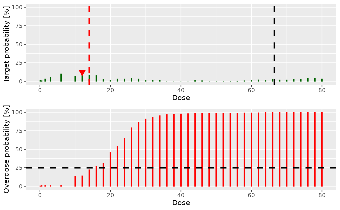
# See the probabilities.
dose_recommendation$probs
#> dose target overdose
#> [1,] 0.1 0.0 1
#> [2,] 0.5 0.0 1
#> [3,] 1.5 0.0 1
#> [4,] 3.0 0.0 1
#> [5,] 6.0 0.2 1
#> [6,] 10.0 0.1 1
#> [7,] 12.0 0.3 1
#> [8,] 14.0 0.1 1
#> [9,] 16.0 0.2 1
#> [10,] 18.0 0.0 1
#> [11,] 20.0 0.0 1
#> [12,] 22.0 0.0 1
#> [13,] 24.0 0.0 1
#> [14,] 26.0 0.0 1
#> [15,] 28.0 0.0 1
#> [16,] 30.0 0.0 1
#> [17,] 32.0 0.0 1
#> [18,] 34.0 0.0 1
#> [19,] 36.0 0.0 1
#> [20,] 38.0 0.0 1
#> [21,] 40.0 0.0 1
#> [22,] 42.0 0.0 1
#> [23,] 44.0 0.0 1
#> [24,] 46.0 0.0 1
#> [25,] 48.0 0.0 1
#> [26,] 50.0 0.0 1
#> [27,] 52.0 0.0 1
#> [28,] 54.0 0.0 1
#> [29,] 56.0 0.0 1
#> [30,] 58.0 0.0 1
#> [31,] 60.0 0.0 1
#> [32,] 62.0 0.0 1
#> [33,] 64.0 0.0 1
#> [34,] 66.0 0.1 1
#> [35,] 68.0 0.0 1
#> [36,] 70.0 0.0 1
#> [37,] 72.0 0.0 1
#> [38,] 74.0 0.0 1
#> [39,] 76.0 0.0 1
#> [40,] 78.0 0.0 1
#> [41,] 80.0 0.0 1
# Joint plot.
print(dose_recommendation$plot)
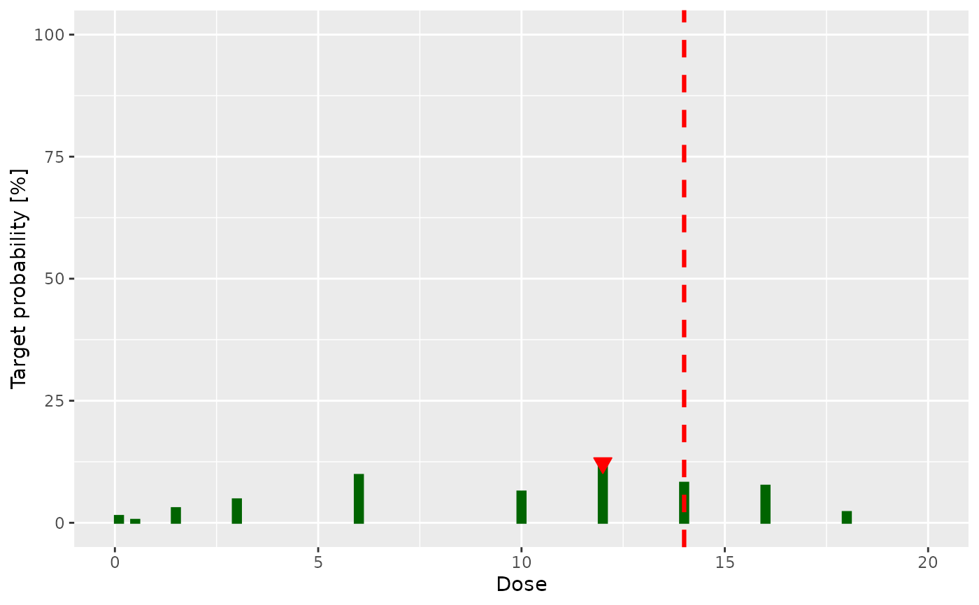
 # Show customization of single plot.
variant1 <- dose_recommendation$singlePlots$plot1 + xlim(0, 20)
print(variant1)
#> Warning: Removed 31 rows containing missing values or values outside the scale range
#> (`geom_bar()`).
#> Warning: Removed 1 row containing missing values or values outside the scale range
#> (`geom_vline()`).
 # }
# Example of usage for `NextBestTD` NextBest class.
my_data <- Data(
x = c(25, 50, 50, 75, 150, 200, 225, 300),
y = c(0, 0, 0, 0, 1, 1, 1, 1),
ID = 1:8,
cohort = c(1L, 2L, 2L, 3L, 4L, 5L, 6L, 7L),
doseGrid = seq(from = 25, to = 300, by = 25)
)
my_model <- LogisticIndepBeta(
binDLE = c(1.05, 1.8),
DLEweights = c(3, 3),
DLEdose = c(25, 300),
data = my_data
)
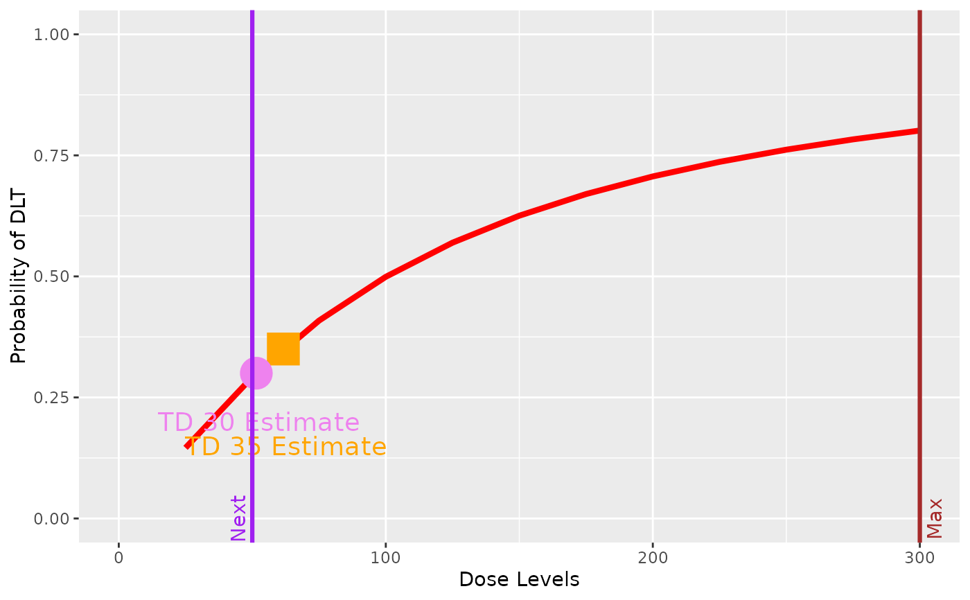
# Target probabilities of the occurrence of a DLT during trial and
# at the end of the trial are defined as 0.35 and 0.3, respectively.
td_next_best <- NextBestTD(prob_target_drt = 0.35, prob_target_eot = 0.3)
# doselimit is the maximum allowable dose level to be given to subjects.
dose_recommendation <- nextBest(
nextBest = td_next_best,
doselimit = max(my_data@doseGrid),
model = my_model,
data = my_data
)
dose_recommendation$next_dose_drt
#> [1] 50
dose_recommendation$plot
 # Example of usage for `NextBestTDsamples` NextBest class.
my_data <- Data(
x = c(25, 50, 50, 75, 150, 200, 225, 300),
y = c(0, 0, 0, 0, 1, 1, 1, 1),
ID = 1:8,
cohort = c(1L, 2L, 2L, 3L, 4L, 5L, 6L, 7L),
doseGrid = seq(from = 25, to = 300, by = 25)
)
my_model <- LogisticIndepBeta(
binDLE = c(1.05, 1.8),
DLEweights = c(3, 3),
DLEdose = c(25, 300),
data = my_data
)
# Set-up some MCMC parameters and generate samples.
my_options <- McmcOptions(burnin = 100, step = 2, samples = 800)
my_samples <- mcmc(my_data, my_model, my_options)
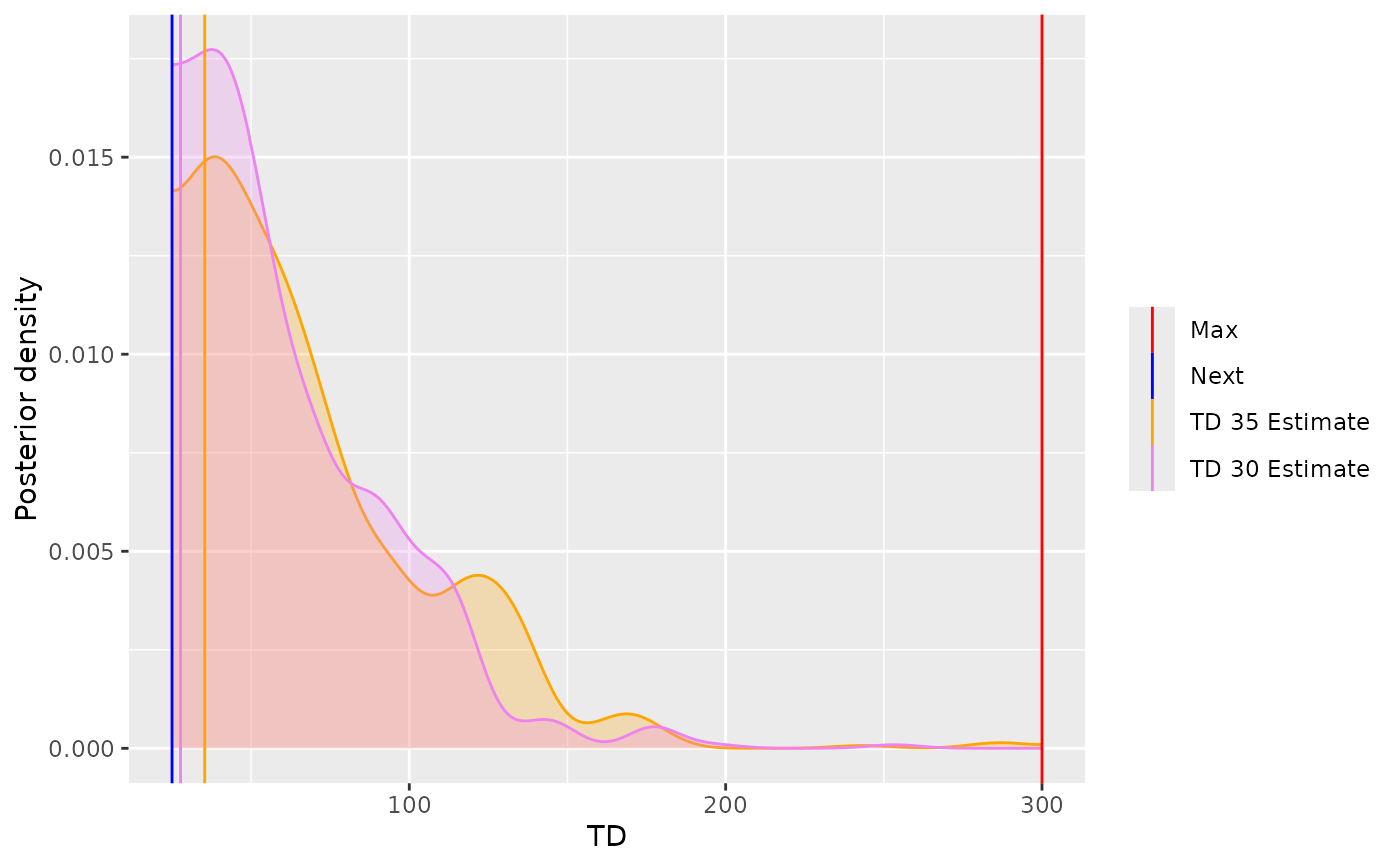
# Target probabilities of the occurrence of a DLT during trial and
# at the end of the trial are defined as 0.35 and 0.3, respectively.
# 'derive' is specified such that the 30% posterior quantile of the TD35 and
# TD30 samples will be used as TD35 and TD30 estimates.
tds_next_best <- NextBestTDsamples(
prob_target_drt = 0.35,
prob_target_eot = 0.3,
derive = function(samples) {
as.numeric(quantile(samples, probs = 0.3))
}
)
# doselimit is the maximum allowable dose level to be given to subjects.
dose_recommendation <- nextBest(
nextBest = tds_next_best,
doselimit = max(my_data@doseGrid),
samples = my_samples,
model = my_model,
data = my_data
)
dose_recommendation$next_dose_drt
#> [1] 50
dose_recommendation$plot
#> Warning: Some data points are outside of `bounds`. Removing them.
#> Warning: Some data points are outside of `bounds`. Removing them.
 # Example of usage for `NextBestMaxGain` NextBest class.
# Create the data.
my_data <- DataDual(
x = c(25, 50, 25, 50, 75, 300, 250, 150),
y = c(0, 0, 0, 0, 0, 1, 1, 0),
ID = 1:8,
cohort = 1:8,
w = c(0.31, 0.42, 0.59, 0.45, 0.6, 0.7, 0.6, 0.52),
doseGrid = seq(25, 300, 25),
placebo = FALSE
)
# 'ModelTox' DLT model, e.g 'LogisticIndepBeta'.
my_model_dlt <- LogisticIndepBeta(
binDLE = c(1.05, 1.8),
DLEweights = c(3, 3),
DLEdose = c(25, 300),
data = my_data
)
# 'ModelEff' efficacy model, e.g. 'Effloglog'.
my_model_eff <- Effloglog(
eff = c(1.223, 2.513),
eff_dose = c(25, 300),
nu = c(a = 1, b = 0.025),
data = my_data
)
# Target probabilities of the occurrence of a DLT during trial and at the
# end of trial are defined as 0.35 and 0.3, respectively.
mg_next_best <- NextBestMaxGain(
prob_target_drt = 0.35,
prob_target_eot = 0.3
)
# doselimit is the maximum allowable dose level to be given to subjects.
dose_recommendation <- nextBest(
nextBest = mg_next_best,
doselimit = 300,
model = my_model_dlt,
model_eff = my_model_eff,
data = my_data
)
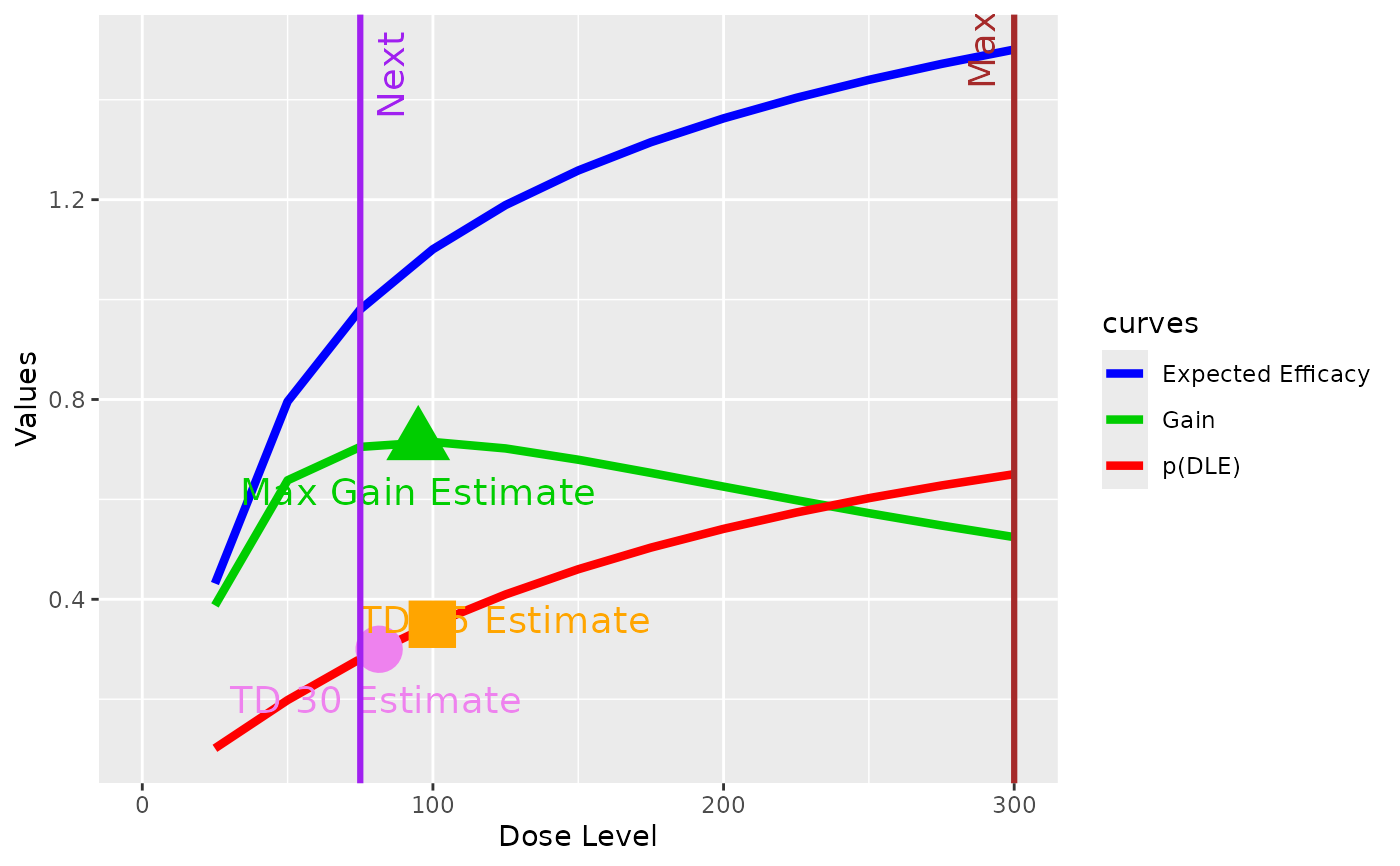
dose_recommendation$next_dose
#> [1] 75
dose_recommendation$plot
 # Example of usage for `NextBestMaxGainSamples` NextBest class.
# Create the data.
my_data <- DataDual(
x = c(25, 50, 25, 50, 75, 300, 250, 150),
y = c(0, 0, 0, 0, 0, 1, 1, 0),
w = c(0.31, 0.42, 0.59, 0.45, 0.6, 0.7, 0.6, 0.52),
ID = 1:8,
cohort = 1:8,
doseGrid = seq(25, 300, 25),
placebo = FALSE
)
# 'ModelTox' DLT model, e.g 'LogisticIndepBeta'.
my_model_dlt <- LogisticIndepBeta(
binDLE = c(1.05, 1.8),
DLEweights = c(3, 3),
DLEdose = c(25, 300),
data = my_data
)
# 'ModelEff' efficacy model, e.g 'Effloglog'.
my_model_effll <- Effloglog(
eff = c(1.223, 2.513),
eff_dose = c(25, 300),
nu = c(a = 1, b = 0.025),
data = my_data
)
# Set-up some MCMC parameters and generate samples from the posterior.
my_options <- McmcOptions(burnin = 5, step = 1, samples = 10)
my_samples_dlt <- mcmc(my_data, my_model_dlt, my_options)
my_samples_effll <- mcmc(my_data, my_model_effll, my_options)
# Target probabilities of the occurrence of a DLT during trial and at the end of
# trial are defined as 0.35 and 0.3, respectively.
# Use 30% posterior quantile of the TD35 and TD30 samples as estimates of TD35
# and TD30.
# Use 50% posterior quantile of the Gstar (the dose which gives the maxim gain value)
# samples as Gstar estimate.
mgs_next_best <- NextBestMaxGainSamples(
prob_target_drt = 0.35,
prob_target_eot = 0.3,
derive = function(samples) {
as.numeric(quantile(samples, prob = 0.3))
},
mg_derive = function(mg_samples) {
as.numeric(quantile(mg_samples, prob = 0.5))
}
)
dose_recommendation <- nextBest(
nextBest = mgs_next_best,
doselimit = max(my_data@doseGrid),
samples = my_samples_dlt,
model = my_model_dlt,
data = my_data,
model_eff = my_model_effll,
samples_eff = my_samples_effll
)
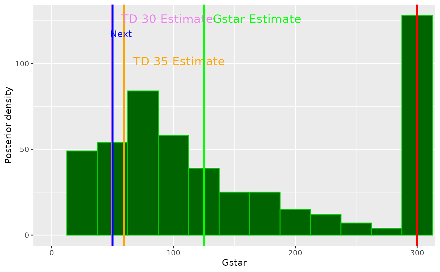
#> [1] "Estimated max gain dose = 300 not within dose grid"
dose_recommendation$next_dose
#> [1] 275
dose_recommendation$plot
 # Now using the 'EffFlexi' class efficacy model:
my_model_effflexi <- EffFlexi(
eff = c(1.223, 2.513),
eff_dose = c(25, 300),
sigma2W = c(a = 0.1, b = 0.1),
sigma2betaW = c(a = 20, b = 50),
rw1 = FALSE,
data = my_data
)
# \donttest{
my_samples_effflexi <- mcmc(my_data, my_model_effflexi, my_options)
dose_recommendation <- nextBest(
nextBest = mgs_next_best,
doselimit = max(my_data@doseGrid),
samples = my_samples_dlt,
model = my_model_dlt,
data = my_data,
model_eff = my_model_effflexi,
samples_eff = my_samples_effflexi
)
dose_recommendation$next_dose
#> [1] 250
dose_recommendation$plot
# }
# Example of usage for `NextBestProbMTDLTE` NextBest class.
# Create the data.
my_data <- Data(
x = c(0.1, 0.5, 1.5, 3, 6, 10, 10, 10),
y = c(0, 0, 0, 0, 0, 0, 1, 0),
ID = 1:8,
cohort = c(0, 1, 2, 3, 4, 5, 5, 5),
doseGrid = c(0.1, 0.5, 1.5, 3, 6, seq(from = 10, to = 80, by = 2))
)
# Initialize the CRM model used to model the data.
my_model <- LogisticLogNormal(
mean = c(-0.85, 1),
cov = matrix(c(1, -0.5, -0.5, 1), nrow = 2),
ref_dose = 56
)
# Set-up some MCMC parameters and generate samples from the posterior.
my_options <- McmcOptions(burnin = 5, step = 1, samples = 10)
my_samples <- mcmc(my_data, my_model, my_options)
# Define the rule for dose increments and calculate the maximum dose allowed.
my_increments <- IncrementsRelative(
intervals = c(0, 20),
increments = c(1, 0.33)
)
next_max_dose <- maxDose(my_increments, data = my_data)
# Define the rule which will be used to select the next best dose
# based on the 'NextBestProbMTDLTE' class.
nb_mtd_lte <- NextBestProbMTDLTE(target = 0.33)
# Calculate the next best dose.
dose_recommendation <- nextBest(
nextBest = nb_mtd_lte,
doselimit = next_max_dose,
samples = my_samples,
model = my_model,
data = my_data
)
# Example of usage for `NextBestProbMTDMinDist` NextBest class.
# Create the data.
my_data <- Data(
x = c(1.5, 1.5, 1.5, 2.5, 2.5, 2.5, 3.5, 3.5, 3.5),
y = c(0, 0, 0, 0, 0, 0, 1, 1, 0),
ID = 1:9,
cohort = c(1, 1, 1, 2, 2, 2, 3, 3, 3),
doseGrid = c(1.5, 2.5, 3.5, 4.5, 6, 7)
)
# Initialize the CRM model used to model the data.
my_model <- my_model <- LogisticKadaneBetaGamma(
theta = 0.3,
xmin = 1.5,
xmax = 7,
alpha = 1,
beta = 19,
shape = 0.5625,
rate = 0.125
)
# Set-up some MCMC parameters and generate samples from the posterior.
my_options <- McmcOptions(burnin = 5, step = 1, samples = 10)
my_samples <- mcmc(my_data, my_model, my_options)
# Define the rule for dose increments and calculate the maximum dose allowed.
my_increments <- IncrementsDoseLevels(levels = 1)
next_max_dose <- maxDose(my_increments, data = my_data)
# Define the rule which will be used to select the next best dose
# based on the 'NextBestProbMTDMinDist' class.
nb_mtd_min_dist <- NextBestProbMTDMinDist(target = 0.3)
# Calculate the next best dose.
dose_recommendation <- nextBest(
nextBest = nb_mtd_min_dist,
doselimit = next_max_dose,
samples = my_samples,
model = my_model,
data = my_data
)
ordinal_data <- .DefaultDataOrdinal()
ordinal_model <- .DefaultLogisticLogNormalOrdinal()
options <- .DefaultMcmcOptions()
# \donttest{
ordinal_samples <- mcmc(ordinal_data, ordinal_model, options)
nextBest(
nextBest = NextBestOrdinal(2L, .DefaultNextBestNCRM()),
samples = ordinal_samples,
doselimit = Inf,
model = ordinal_model,
data = ordinal_data
)
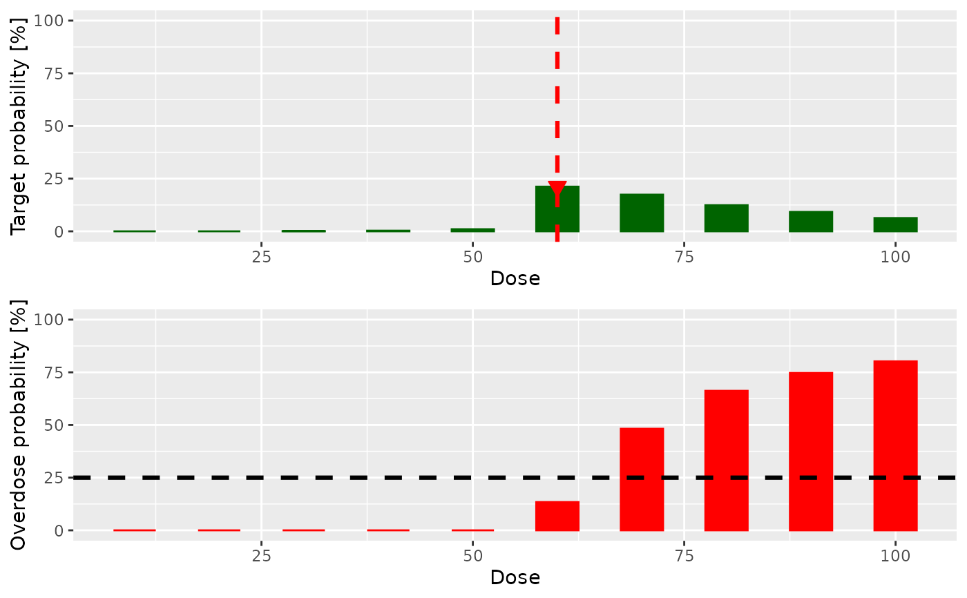 #> $value
#> [1] 60
#>
#> $plot
#>
#> $singlePlots
#> $singlePlots$plot1
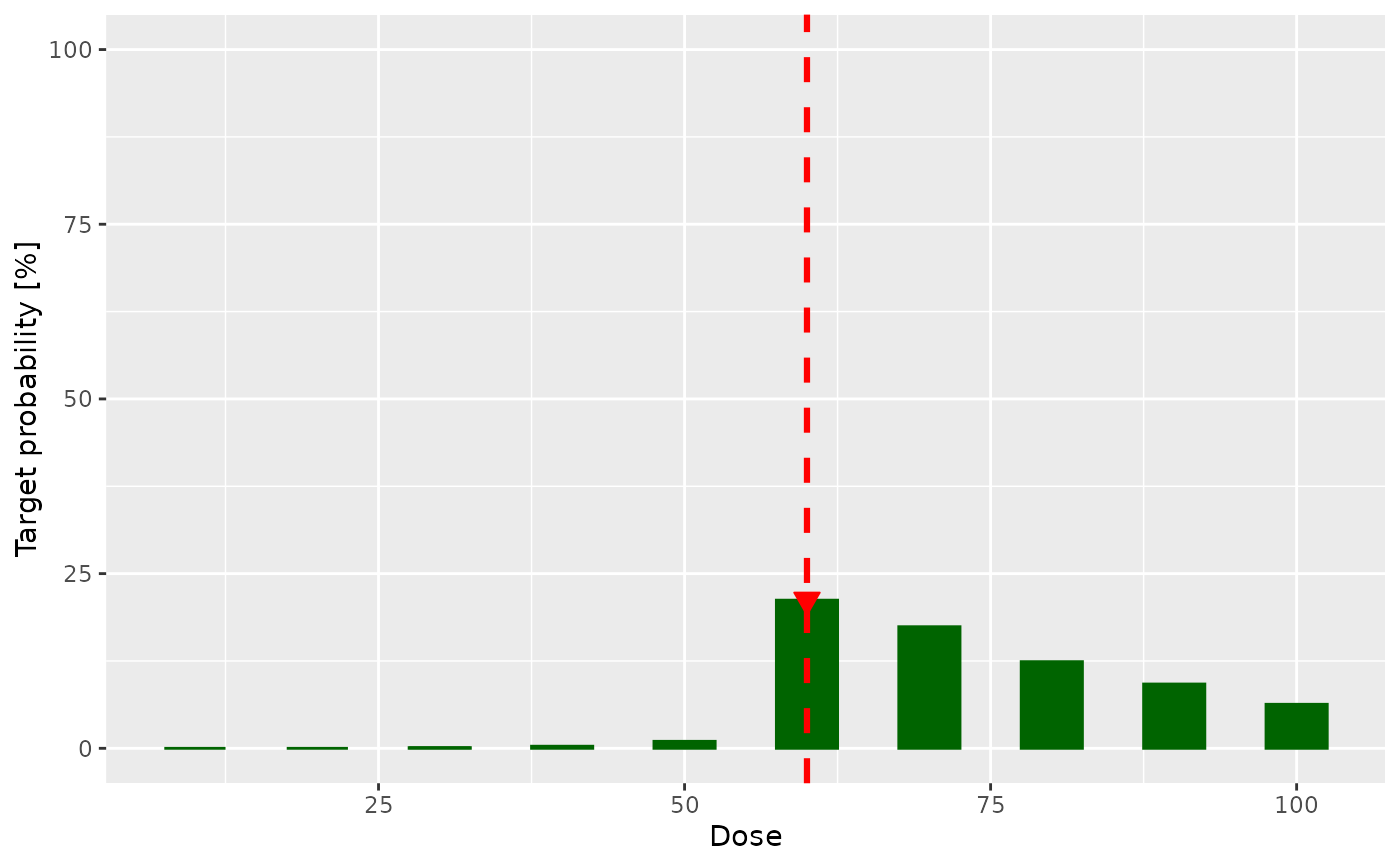 #>
#> $singlePlots$plot2
#>
#>
#> $probs
#> dose target overdose
#> [1,] 10 0.000 0.000
#> [2,] 20 0.000 0.000
#> [3,] 30 0.001 0.000
#> [4,] 40 0.003 0.000
#> [5,] 50 0.025 0.001
#> [6,] 60 0.206 0.160
#> [7,] 70 0.170 0.476
#> [8,] 80 0.141 0.639
#> [9,] 90 0.123 0.728
#> [10,] 100 0.081 0.799
#>
# }
ordinal_data <- .DefaultDataOrdinal()
ordinal_model <- .DefaultLogisticLogNormalOrdinal()
options <- .DefaultMcmcOptions()
# \donttest{
ordinal_samples <- mcmc(ordinal_data, ordinal_model, options)
nextBest(
nextBest = NextBestOrdinal(2L, .DefaultNextBestNCRM()),
samples = ordinal_samples,
doselimit = Inf,
model = ordinal_model,
data = ordinal_data
)
#>
#> $singlePlots$plot2
#>
#>
#> $probs
#> dose target overdose
#> [1,] 10 0.000 0.000
#> [2,] 20 0.000 0.000
#> [3,] 30 0.001 0.000
#> [4,] 40 0.003 0.000
#> [5,] 50 0.025 0.001
#> [6,] 60 0.206 0.160
#> [7,] 70 0.170 0.476
#> [8,] 80 0.141 0.639
#> [9,] 90 0.123 0.728
#> [10,] 100 0.081 0.799
#>
# }
ordinal_data <- .DefaultDataOrdinal()
ordinal_model <- .DefaultLogisticLogNormalOrdinal()
options <- .DefaultMcmcOptions()
# \donttest{
ordinal_samples <- mcmc(ordinal_data, ordinal_model, options)
nextBest(
nextBest = NextBestOrdinal(2L, .DefaultNextBestNCRM()),
samples = ordinal_samples,
doselimit = Inf,
model = ordinal_model,
data = ordinal_data
)
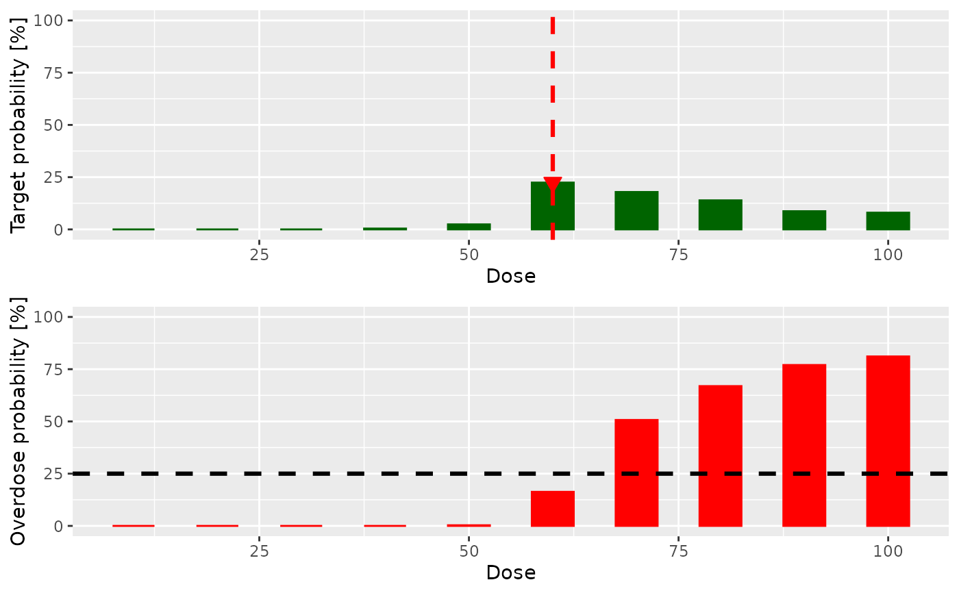 #> $value
#> [1] 60
#>
#> $plot
#>
#> $singlePlots
#> $singlePlots$plot1
 #>
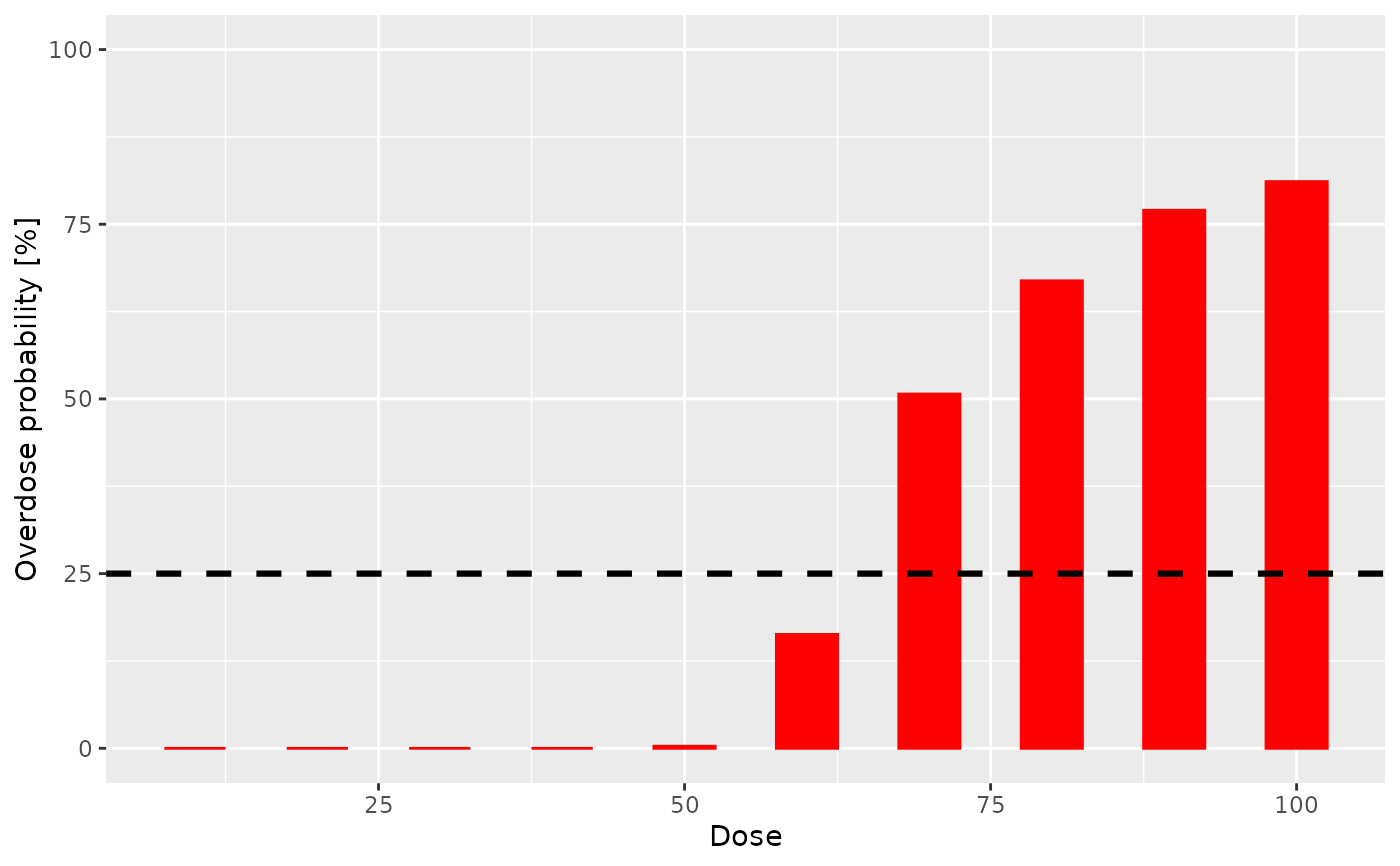
#> $singlePlots$plot2
#>
#> $singlePlots$plot2
 #>
#>
#> $probs
#> dose target overdose
#> [1,] 10 0.000 0.000
#> [2,] 20 0.000 0.000
#> [3,] 30 0.000 0.000
#> [4,] 40 0.004 0.000
#> [5,] 50 0.014 0.001
#> [6,] 60 0.218 0.127
#> [7,] 70 0.193 0.480
#> [8,] 80 0.122 0.666
#> [9,] 90 0.099 0.747
#> [10,] 100 0.071 0.796
#>
# }
#>
#>
#> $probs
#> dose target overdose
#> [1,] 10 0.000 0.000
#> [2,] 20 0.000 0.000
#> [3,] 30 0.000 0.000
#> [4,] 40 0.004 0.000
#> [5,] 50 0.014 0.001
#> [6,] 60 0.218 0.127
#> [7,] 70 0.193 0.480
#> [8,] 80 0.122 0.666
#> [9,] 90 0.099 0.747
#> [10,] 100 0.071 0.796
#>
# }
