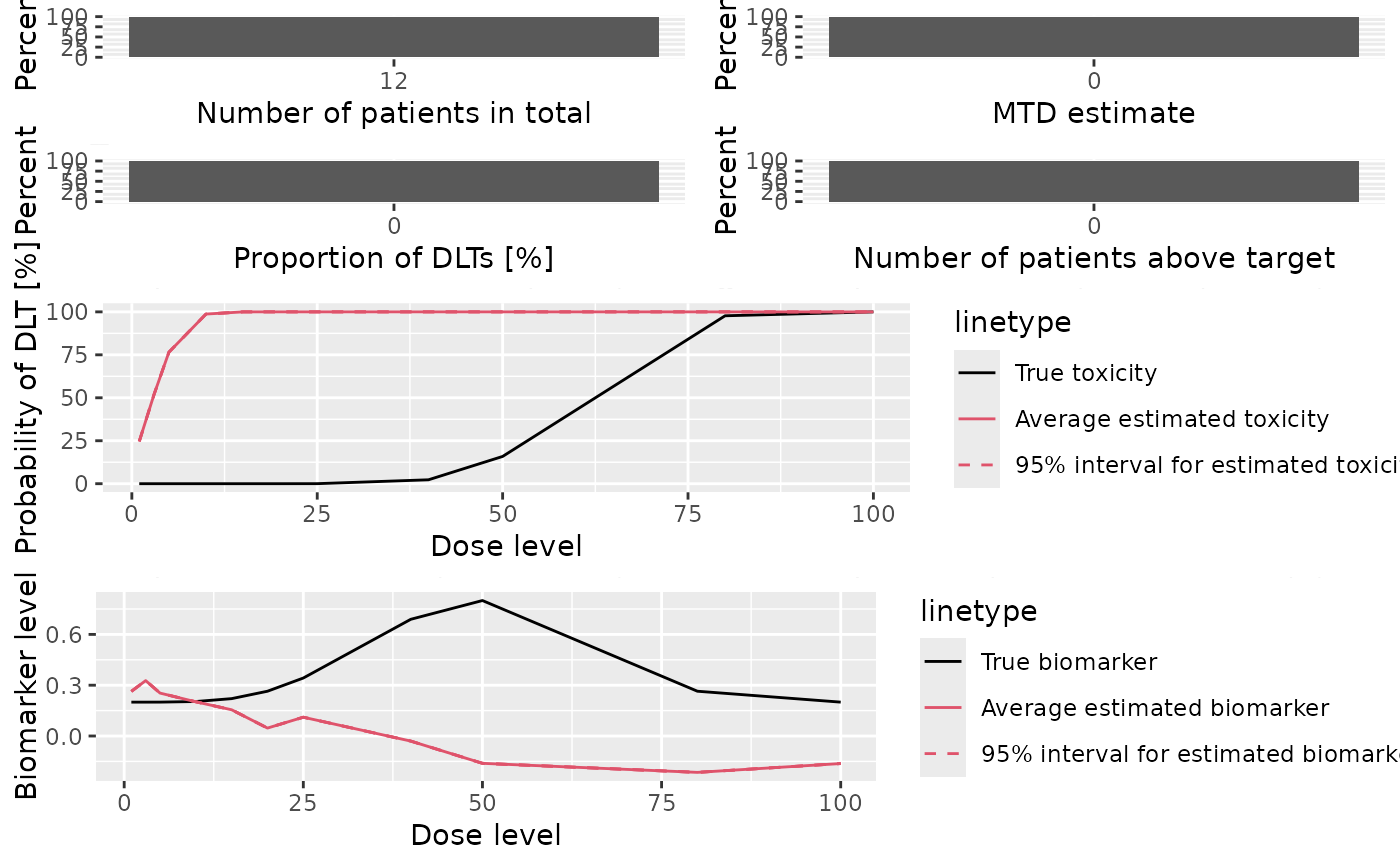
Plot summaries of the dual-endpoint design simulations

This plot method can be applied to DualSimulationsSummary objects in order to summarize them graphically. Possible type of plots at the moment are those listed in plot,SimulationsSummary,missing-method plus:

meanBiomarkerFit

Plot showing the average fitted dose-biomarker curve across the trials, together with 95% credible intervals, and comparison with the assumed truth (as specified by the trueBiomarker argument to summary,DualSimulations-method)

You can specify any subset of these in the type argument.

Usage

# S4 method for class 'DualSimulationsSummary,missing'
plot(
  x,
  y,
  type = c("nObs", "doseSelected", "propDLTs", "nAboveTarget", "meanFit",
    "meanBiomarkerFit"),
  ...
)

Arguments

x

the DualSimulationsSummary object we want to plot from

y

missing

type

the types of plots you want to obtain.

...

not used

Value

A single ggplot object if a single plot is asked for, otherwise a gridExtra{gTree} object.

Examples

# Define the dose-grid.
emptydata <- DataDual(doseGrid = c(1, 3, 5, 10, 15, 20, 25, 40, 50, 80, 100))


# Initialize the CRM model.
my_model <- DualEndpointRW(
  mean = c(0, 1),
  cov = matrix(c(1, 0, 0, 1), nrow = 2),
  sigma2betaW = 0.01,
  sigma2W = c(a = 0.1, b = 0.1),
  rho = c(a = 1, b = 1),
  rw1 = TRUE
)


# Choose the rule for selecting the next dose.
my_next_best <- NextBestDualEndpoint(
  target = c(0.9, 1),
  overdose = c(0.35, 1),
  max_overdose_prob = 0.25
)

# Choose the rule for the cohort-size.
my_size1 <- CohortSizeRange(
  intervals = c(0, 30),
  cohort_size = c(1, 3)
)
my_size2 <- CohortSizeDLT(
  intervals = c(0, 1),
  cohort_size = c(1, 3)
)
my_size <- maxSize(my_size1, my_size2)

# Choose the rule for stopping.
my_stopping4 <- StoppingTargetBiomarker(
  target = c(0.9, 1),
  prob = 0.5
)
# Only 10 patients here for illustration!
my_stopping <- my_stopping4 | StoppingMinPatients(10) | StoppingMissingDose()

# Choose the rule for dose increments.
my_increments <- IncrementsRelative(
  intervals = c(0, 20),
  increments = c(1, 0.33)
)

# Initialize the design.
my_design <- DualDesign(
  model = my_model,
  data = emptydata,
  nextBest = my_next_best,
  stopping = my_stopping,
  increments = my_increments,
  cohort_size = CohortSizeConst(3),
  startingDose = 3
)

# Define scenarios for the TRUE toxicity and efficacy profiles.
beta_mod <- function(dose, e0, eMax, delta1, delta2, scal) {
  maxDens <- (delta1^delta1) * (delta2^delta2) / ((delta1 + delta2)^(delta1 + delta2))
  dose <- dose / scal
  e0 + eMax / maxDens * (dose^delta1) * (1 - dose)^delta2
}



true_biomarker <- function(dose) {
  beta_mod(dose, e0 = 0.2, eMax = 0.6, delta1 = 5, delta2 = 5 * 0.5 / 0.5, scal = 100)
}

true_tox <- function(dose) {
  pnorm((dose - 60) / 10)
}

# Draw the TRUE profiles.
par(mfrow = c(1, 2))
curve(true_tox(x), from = 0, to = 80)
curve(true_biomarker(x), from = 0, to = 80)

# Run the simulation on the desired design.
# We only generate 1 trial outcome here for illustration, for the actual study.
# For illustration purpose we will use 5 burn-ins to generate 20 samples,
# this should be increased of course.
my_sims <- simulate(
  object = my_design,
  trueTox = true_tox,
  trueBiomarker = true_biomarker,
  sigma2W = 0.01,
  rho = 0,
  nsim = 1,
  parallel = FALSE,
  seed = 3,
  startingDose = 6,
  mcmcOptions = McmcOptions(
    burnin = 5,
    step = 1,
    samples = 20
  )
)

# Plot the summary of the Simulations.
plot(summary(my_sims,
  trueTox = true_tox,
  trueBiomarker = true_biomarker
))